

Project and Quality Management is a mandatory core topic in Leaving Certificate Technology. It gives you the planning, scheduling, and analytical tools to take an idea from initial design to a reliable finished artefact within set constraints of time, cost, and materials. In the written paper, this material is examined in Section A (core short questions) and Section B (core long questions). In the coursework project, which accounts for 50% of the total examination marks, project planning, scheduling (Gantt charts, critical path networks), product costings, and reliability testing must be documented directly in your design folio.
Projects, Goals, and the Triple Constraint
A project is a temporary, one-off undertaking designed to achieve a defined objective within finite resources. It has an identifiable start and finish, which separates it from continuous factory operations like mass-producing identical screws.
Every technology project operates under the triple constraint, often called the three pillars of project management:
- Time: The project must meet a strict deadline, such as the SEC coursework submission date.
- Cost: Total expenditure on materials, components, tooling, and energy must stay within budget.
- Quality: The finished artefact must satisfy defined functional, structural, safety, and aesthetic standards.
These three constraints continuously pull against each other. If you compress your schedule to finish earlier, you often have to buy expensive pre-assembled sub-systems (raising costs) or rush assembly (lowering quality). If you cut material costs by buying cheap parts, the mechanism may fail during testing. Beyond these three pillars, school workshop projects must also manage practical constraints including tool availability, personal skill levels, and workshop safety regulations.
A project begins with a design brief and develops into a measurable design specification. A vague goal such as "make something for older people" provides no clear standard of success. An effective goal defines clear operational boundaries: "Design and manufacture an automated pill dispenser with audio-visual alerts and a rotating carousel for an older person, completed within eight weeks for under €40."
Work Breakdown Structure and Gantt Charts
Before picking up tools, you must organise the work. A Work Breakdown Structure (WBS) decomposes the overall project hierarchically into manageable stages and discrete tasks. It does not record dates or durations; it acts as a complete checklist of every task, so nothing is forgotten.
Assistive Pill Dispenser
├── 1. Research and Specification
│   ├── 1.1 Investigate user needs and anthropometrics
│   ├── 1.2 Formulate measurable design specifications
│   └── 1.3 Produce circuit schematics and CAD drawings
├── 2. Procurement and Costing
│   ├── 2.1 Calculate materials and component list costings
│   └── 2.2 Procure motor, microcontroller, and acrylic
├── 3. Production and Realisation
│   ├── 3.1 Laser-cut acrylic chassis plates
│   ├── 3.2 Solder PCB circuit and download program
│   └── 3.3 Assemble drive motor, gearing, and carousel
└── 4. Testing and Evaluation
    ├── 4.1 Execute 100-cycle latch and motor reliability test
    └── 4.2 Compare planned against actual timeline
Once tasks, durations, and dependencies are defined, you schedule them on a Gantt chart.
Reading and Interpreting a Gantt Chart
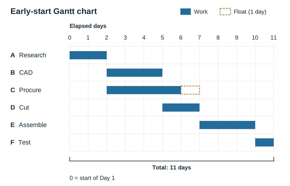
A Gantt chart lists tasks vertically down the left and displays time horizontally across the top. Each task appears as a horizontal bar:
- Task duration: Count the number of time units covered by the bar.
- Start and finish: The left-hand edge marks the start time; the right-hand edge marks the completion time.
- Concurrent (parallel) tasks: Bars that overlap vertically take place at the same time (for example, soldering the circuit while waiting for laser-cut chassis panels to arrive).
- Total project duration: Measured from the left edge of the earliest task to the right edge of the final completed task.
- Milestone: A significant checkpoint with zero duration, plotted as a diamond or vertical line (e.g. "Circuit prototype verified").
- Monitoring progress: A second, shaded bar drawn beneath the planned bar shows actual progress. A shaded bar that ends short of the current date indicates the activity is behind schedule.
Network Diagrams, Critical Path Analysis, and Float
For projects with complex dependencies, a network diagram maps the exact flow of activities. The fundamental rule is straightforward: an activity cannot start until all its immediate predecessors are finished.
Drawing the Network Diagram
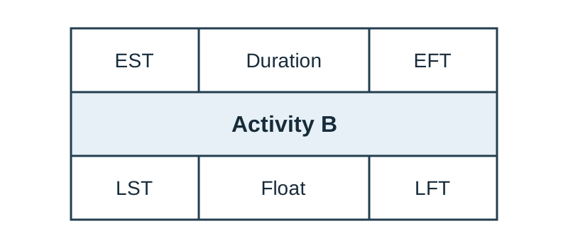
Each activity is drawn as a standardized box (node). Keep the same six-cell layout for every box so the examiner can read your numbers easily:
To construct and analyse the network:
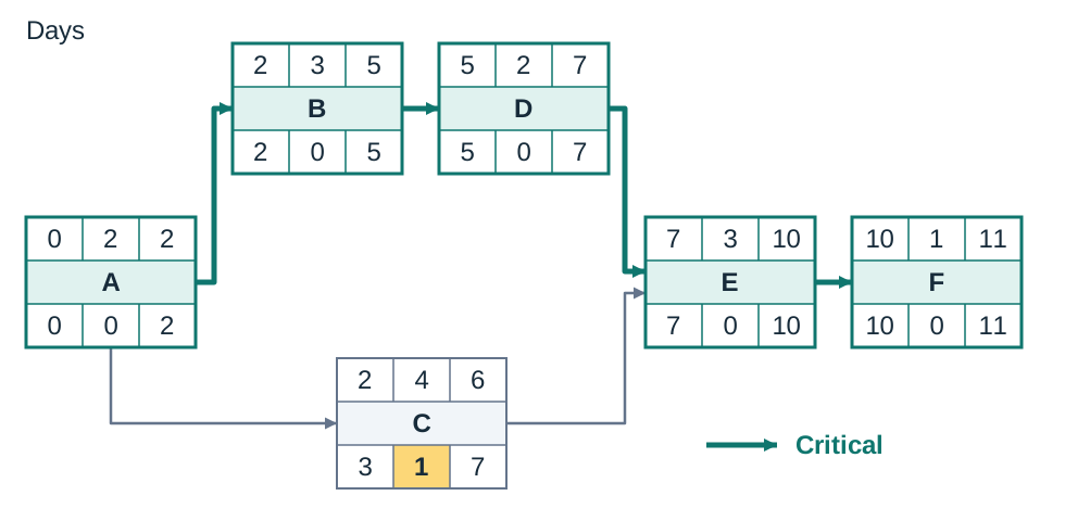
- Draw a node for each activity from left to right, joining them with arrows to represent dependencies. An arrow from A to B means "B cannot start until A is finished".
- Times are measured from project commencement. An Earliest Start Time (EST) of 0 means the activity begins at the start of Day 1.
- Forward Pass (Left to Right): Calculate the earliest times. . When two or more activities feed into one activity, that activity cannot start until all of them are finished, so its EST equals the largest incoming EFT.
- Backward Pass (Right to Left): Set the final activity's Latest Finish Time (LFT) equal to the project duration. Calculate latest times: . When an activity feeds into multiple successors, its LFT equals the smallest outgoing LST.
- Calculate Total Float: Write the float into the bottom-centre cell using .
- Identify the critical path—the continuous chain of activities with zero float. Mark it with bold or double arrows and state the total project duration.
The critical path is the longest sequence of dependent tasks through the network. Because every task on it must be done in order, with no delay, it fixes the shortest time in which the whole project can be completed. Critical activities have zero float, so any delay to one of them delays the whole project.
Quality Principles and Attributes
In technology, quality is defined as fitness for purpose—how effectively a product satisfies the specified needs and reasonable expectations of the user. Quality does not mean luxury or a high price. A cheap moulded plastic pillbox that latches securely and keeps medication dry is a high-quality product.
Two closely linked terms are frequently examined:
- Quality Control (QC) is the detection of faults. It involves inspecting, measuring, and testing materials, parts, and finished products to find those that do not meet the specification, so they can be reworked or scrapped. Example: gauging the diameter of every tenth turned bush with a vernier calliper.
- Quality Assurance (QA) is the prevention of faults. It is the complete system of planned procedures, documented work instructions, staff training, machine calibration, and supplier approval put in place so defects are not produced in the first place. Example: establishing a standard temperature-controlled soldering procedure and training technicians before production starts.
A simple rule for the exam: quality control inspects the product; quality assurance manages the process.
The Core Quality Attributes
- Performance: How well the product carries out its primary function (e.g. motor delivers sufficient torque to rotate the carousel under load).
- Reliability: The probability that a device will perform without failure under stated conditions for a specified period.
- Durability: The length of active operating life before physical wear or fatigue makes the product unserviceable.
- Conformance: The precision with which a manufactured part adheres to engineering drawings, dimensions, and specified tolerances.
- Safety: The protection of the user from electric shock, sharp edges, trapping hazards, or toxic materials during normal use and reasonable misuse.
- Aesthetics and Ergonomics: Visual appeal, clean surface finish, comfortable grip, and intuitive layout of controls.
- Features: Secondary characteristics that supplement the basic function and add value (e.g. an alert that vibrates as well as beeps for a hearing-impaired user).
- Perceived Quality: The impression of quality formed from brand reputation, customer reviews, packaging, and tactile surface finish.
- Serviceability: The ease with which parts can be inspected, maintained, or replaced.
- Value for Money: The balance between initial purchase plus running costs and the functional benefits delivered.
The Product Life Cycle and Product Costing
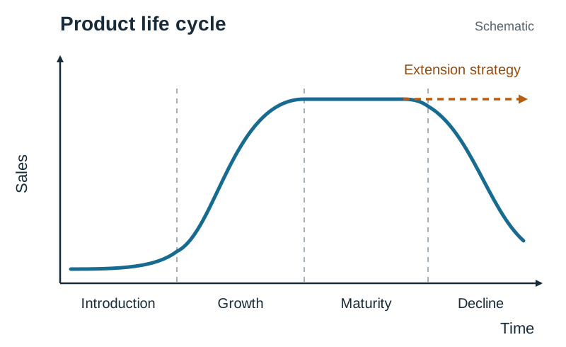
The commercial life of a product follows the product life cycle, which graphs sales volume or revenue against time.
Drawing and Labelling the Graph
- Axes: Label the vertical axis Sales (volume or revenue) and the horizontal axis Time.
- Curve Shape: The curve starts low and flat, rises steeply, plateaus at its peak, and then curves downward—an S-shape followed by a decline.
- The Four Stages: Divide the curve using vertical dashed lines and label the four stages underneath in order: Introduction, Growth, Maturity, and Decline.
- Examiner details: A pre-launch research and development (R&D) phase with zero sales and high costs is often shown before Introduction. An arrow extending from the maturity plateau can be labelled "extension strategy" (e.g. adding new features or cosmetic redesign to delay decline).
Do not confuse the product life cycle (a market curve of sales against time) with life cycle analysis (LCA, which evaluates environmental impacts from raw material extraction through manufacture and use to final disposal).
| Life Cycle Stage | Sales Pattern | Market and Manufacturing Realities |
|---|---|---|
| 1. Introduction | Low sales | High R&D and launch costs. Production runs are small while initial assembly bugs are resolved. Sound quality attributes like reliability and safety are critical to build user confidence and positive initial reviews. |
| 2. Growth | Rising rapidly | Customer acceptance spreads. Production volume ramps up, and economies of scale reduce unit manufacturing costs. High quality and conformance drive repeat purchases and strong market share growth. |
| 3. Maturity | Peak and plateau | Market is saturated. Competition is intense. Sustaining high quality, refining aesthetics, or adding new features helps defend market share and extend the product life cycle. |
| 4. Decline | Falling sales | Demand drops due to technological advances, competing superior designs, or changing consumer habits. Quality degradation accelerates decline. The product is discounted, phased out, or replaced. |
Quality, Market Share, and Manufacturing Costs
Market share is a firm's sales expressed as a percentage of total sales across that entire product market:
Quality, market share, and manufacturing costs are directly linked:
- Quality and market share: A product whose quality attributes satisfy user needs builds a strong reputation, attracting more customers and increasing market share. This extends the profitable growth and maturity stages. Products with poor quality or early failures suffer negative reviews, lose market share, and decline rapidly.
- Market share and manufacturing costs: Achieving a larger market share requires higher production volumes. Higher volumes create economies of scale, spreading fixed tooling, equipment, and R&D costs over more units, which significantly reduces the unit manufacturing cost.
- Quality and manufacturing costs: Investing early in quality prevention reduces internal failure costs (such as scrap and rework) and external failure costs (such as warranty replacements and customer complaints), lowering the overall cost of manufacture.
Identifying, Classifying, and Estimating Product Costs
In folio production planning and written exams, product costs are classified into four headings:
- Direct costs: Traced directly to one specific product (e.g. acrylic sheet, microcontroller, motor, operator assembly labour).
- Indirect costs (overheads): Shared factory operating expenses that cannot be assigned to one single part (e.g. workshop heating, lighting, machine depreciation, rent).
- Fixed costs: Expenses that remain unchanged regardless of output volume (e.g. CAD software licences, injection mould tooling).
- Variable costs: Expenses that rise and fall directly with output volume (e.g. raw polymers, electronic components, packaging).
Worked costing example: A batch of 50 pill dispensers consumes €6.20 of acrylic and €9.40 of electronic components per unit. Direct assembly labour is 0.75 hours per unit at €14.00 per hour. Shared workshop overheads allocated to the batch total €260. Find the unit cost.
- Direct materials per unit = €6.20 + €9.40 = €15.60
- Direct labour per unit = 0.75 h × €14.00/h = €10.50
- Overhead per unit = €260 ÷ 50 = €5.20
- Unit cost = €15.60 + €10.50 + €5.20 = €31.30
Quality Tools, Data Presentation, and the Deming Cycle
Quality management uses data-driven problem solving rather than guesswork. Continuous process improvement is structured around the Deming Cycle (PDCA or PDSA): Plan, Do, Study (or Check), and Act.
A practical workshop example illustrates the cycle:
- Plan: A tally chart records 12 dry solder joints across 50 completed boards. The plan is to raise the soldering iron temperature from 300 °C to 340 °C and apply flux cored solder.
- Do: Solder a test batch of 20 circuit boards at 340 °C.
- Study / Check: Inspect the trial batch; only 1 dry joint occurs in 20 boards, down from 24% to 5%.
- Act: Standardise 340 °C in the written workshop procedure and train all students; then restart the cycle to address the next most frequent defect.
Core Quality Problem-Solving Tools
- Cause-and-Effect Diagram (Fishbone or Ishikawa Diagram): Brainstorms potential root causes of a specific fault. The fault (effect) sits at the right-hand spine head. Brainstormed causes branch out into the 4 Ms: Materials, Methods, Machines, and Manpower (People).
- Checksheet / Tally Chart: A structured recording sheet used at the bench to log defect frequencies as they occur.
- Bar Chart: Visual rectangular bars comparing defect occurrences across categories.
- Pareto Chart: A bar chart where defect categories are arranged in descending order of frequency. It applies the 80/20 rule, showing that a vital few causes create the majority of problems, ensuring effort is targeted at the tallest bars first.
- Scatter Diagram: Plots paired coordinates to detect whether two variables are related. Points sloping upward left-to-right show positive correlation; downward show negative correlation; a random cloud shows no correlation. Correlation indicates an association, but controlled testing is needed to confirm causation.
Statistical Measures
- Mean: (arithmetic average of measurements).
- Median: The middle value when readings are ranked in numerical order (average the two central numbers if is even).
- Mode: The value occurring with greatest frequency.
- Range: (measures dimensional spread and process variability).
Degradation and the Cost of Quality
Degradation is the reduction in a product's intended quality attributes. It occurs across two phases:
Degradation During Design and Realisation
Inaccurate marking out, blunt cutters, warped sheet stock, or component overheating during soldering degrade the artefact below its design intent. Quality loss is cumulative: tiny dimensional deviations on individual parts compound during final assembly, leading to binding mechanisms or misaligned casings.
Degradation in Operational Use
Physical deterioration in service caused by friction and mechanical wear, cyclic fatigue loading, atmospheric corrosion of metals, UV embrittlement of polymers, or chemical decay of battery cells.
Where a higher numerical value represents superior quality (battery operational life, load capacity, cycle count), degradation is calculated as:
Worked degradation example: A latch mechanism specified to operate for 500 cycles without failure jams permanently after 420 cycles. Degradation = .
For a physical dimension, quantify degradation as dimensional deviation from the nominal size: . If a locating pin specified as is turned to , the deviation is , exceeding tolerance by .
The Cost of Quality (CoQ) Framework
Quality expenditures fall into four distinct categories:
- Prevention Costs (Cost of Conformance): Money spent to stop defects before manufacture. Examples: operator training, design reviews, CAD simulation, and preventative tool maintenance.
- Appraisal Costs (Cost of Conformance): Money spent checking, measuring, and testing materials and parts to confirm compliance with specifications. Examples: calliper tolerance checks, multimeter testing of circuits, and incoming batch inspection.
- Internal Failure Costs (Cost of Non-conformance): Financial losses from defects caught before dispatch. Examples: scrapped acrylic offcuts, desoldering and repairing bridged circuit joints, and machine downtime.
- External Failure Costs (Cost of Non-conformance): Losses incurred after the customer receives a defective product. Examples: warranty replacements, customer compensation, product recalls, and catastrophic loss of commercial reputation.
Investing in prevention is always the most economical policy. Eliminating a flaw on a CAD drawing costs pennies; fixing it on the workshop floor costs tens of euros; recalling thousands of defective products from customers costs tens of thousands of euros.
Reliability Engineering and Testing Programmes
Reliability is the probability that an engineering component or system will perform its required function under specified operating conditions for a stated period without failure. Running a mechanism successfully once demonstrates functionality, not reliability.
Reliability features are the specific design details that stop a product failing in normal use. Key examples in simple products include:
- Enclosure sealing: Using gaskets or close-fitting housings to keep moisture and dust out of internal circuits.
- Strain relief: Securing cables where they enter an enclosure (e.g. with a rubber grommet or clamp) so pulling the lead cannot snap wires off internal joints.
- Component derating: Operating parts well below their maximum electrical or thermal ratings (such as running a motor or resistor below peak capacity) to prevent overheating.
- Protective cut-outs: Including a fuse or thermal switch to protect circuits from overload.
- Low-battery warning: Providing a sensor or indicator alert before power drops completely, preventing unexpected stoppage.
- Minimising moving parts: Reducing linkages and gears, since every extra part is another potential point of failure.
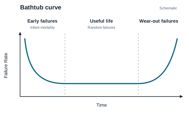
Across a product population, failure behaviour over time follows the Bathtub Curve:
- Sketching the curve: Draw the vertical axis as Failure Rate and the horizontal axis as Time. Draw a steep falling curve on the left, a long flat low section across the middle, and a steeply rising curve on the right. Label the two axes and the three distinct regions:
- Early Failures (Infant Mortality / Burn-in): A high initial failure rate that drops quickly. Caused by manufacturing defects, poor solder joints, or faulty components. Manufacturers eliminate these before customer delivery using burn-in testing (running units under elevated electrical or thermal stress for a trial period).
- Useful Life (Random Failures): A prolonged period with a low, constant failure rate. Failures occur randomly due to unexpected operating overloads rather than design defects.
- Wear-out Failures: An increasing failure rate at the end of product life as components reach their physical fatigue limits (gear teeth wear, bearings pit, plastics degrade). Prevented by scheduled maintenance and replacing worn components.
Information Required for Analysing Reliability
To evaluate reliability, record six parameters: (1) Sample size tested (), (2) Total operating time or cycles run, (3) Number of failures, (4) Exact time or cycle of each failure, (5) Specific failure mode (how and why it broke), and (6) Pre-agreed definition of failure.
- Reliability:
- Failure Rate ():
- Mean Time Between Failures (MTBF):
Worked reliability example: 10 alarm units are run on test for 400 hours each. During the test, 2 units fail.
- Total operating time =
- MTBF =
- Failure rate
- Reliability =
Devising a Seven-Step Reliability Testing Programme
- Define failure criteria: State measurable limits (e.g. motor stall, latch jamming, or gear slip under a 250 g load).
- Select representative sample: Choose a set number of units from the production batch.
- Set controlled test conditions: Fix voltage, temperature, cyclic speed, and load.
- Record baseline data: Log starting dimensions, operating current, and speed.
- Execute and monitor testing: Run automated cycling, recording the exact cycle and failure mode of any breakdown.
- Analyse data: Calculate MTBF and failure rates; use a fishbone diagram to trace root causes.
- Implement redesign and retest: Upgrade weak materials or integrate reliability features (such as adding cable strain relief, protective sealing, or component derating), and repeat testing to confirm reliability gains.
Key terms
- Project
- A temporary, one-off undertaking with a defined start, finish, specific objectives, and finite resources of time, cost, and personnel.
- Triple Constraint
- The interactive balance between time, cost, and quality in project management, where altering one constraint directly affects the other two.
- Work Breakdown Structure (WBS)
- A hierarchical planning tool that decomposes the total scope of a project into manageable stages and discrete tasks.
- Gantt Chart
- A horizontal bar chart showing scheduled tasks against a timeline, displaying task start dates, durations, and concurrent activities.
- Critical Path
- The longest continuous sequence of dependent tasks through a project network, which determines the minimum possible time to complete the project.
- Total Float
- The spare time an activity can be delayed without delaying the project completion date, calculated as Float = LST − EST = LFT − EFT.
- Quality Control (QC)
- The operational process of inspecting, measuring, and testing products to detect defects and verify conformance to specifications.
- Quality Assurance (QA)
- The planned, systematic process of managing procedures, training, and production methods to prevent defects from occurring.
- Conformance
- The precision with which a manufactured component adheres to established dimensions, engineering drawings, and tolerance limits.
- Deming Cycle
- A four-stage continuous improvement cycle consisting of Plan, Do, Study (or Check), and Act (PDCA/PDSA).
- Cause-and-Effect Diagram
- A fishbone (Ishikawa) diagram used to brainstorm and categorise root causes of a quality fault under Materials, Methods, Machines, and Manpower.
- Prevention Costs
- Expenditures incurred to stop defects before manufacture, such as staff training, design refinement, supplier qualification, and maintenance.
- Appraisal Costs
- Expenses incurred by inspecting, checking, and testing parts and assemblies to verify standards.
- Internal Failure Costs
- Financial losses from defects caught before a product reaches the customer, including scrap, rework, and re-inspection.
- External Failure Costs
- Financial losses from defects discovered after delivery to the customer, including warranty claims, recalls, and reputation damage.
- Degradation
- The loss or reduction of a product's intended quality attributes occurring during manufacture or throughout operational life.
- Reliability
- The probability that a product will perform its required function without failure under stated operating conditions for a specified period.
- Bathtub Curve
- A graph of failure rate against time exhibiting three distinct stages: early failures (infant mortality), useful life (random), and wear-out.
- Burn-in Testing
- Pre-dispatch testing of components under elevated electrical or thermal stress to trigger and weed out infant mortality defects.
- Mean Time Between Failures (MTBF)
- The average operating time elapsed between failures in a repairable system, calculated as total operating time divided by number of failures.
Check yourself
Name the two axes of a product life cycle graph and the four stages along the time axis in correct order.
Vertical axis: Sales (volume or revenue); Horizontal axis: Time. The four stages are Introduction, Growth, Maturity, and Decline.
A Gantt chart shows Task A over weeks 1–3, Task B over weeks 2–5, and Task C over weeks 5–6. Which tasks run concurrently and what is the total duration?
Tasks A and B run concurrently during weeks 2–3; Tasks B and C run concurrently during week 5. The total project duration is 6 weeks.
Classify each expenditure: (a) operator soldering training, (b) vernier calliper inspection of bosses, (c) scrapped acrylic cutouts, (d) customer product recall notice.
(a) Prevention cost, (b) Appraisal cost, (c) Internal failure cost, (d) External failure cost.
Activity D depends on Activity B (EFT = 6 days) and Activity C (EFT = 9 days). What is the EST of Activity D?
9 days. Activity D cannot begin until all predecessors are complete (the largest incoming EFT).
An activity has an EST of Day 5, a duration of 4 days, and an LFT of Day 12. Calculate its float.
3 days. (LST = LFT − Duration = 12 − 4 = 8. Float = LST − EST = 8 − 5 = 3 days).
State the four stages of the continuous improvement Deming Cycle in correct sequence.
Plan, Do, Study (or Check), Act.
Name the four standard categories branching off the central spine of a cause-and-effect (fishbone) diagram.
Materials, Methods, Machines, and Manpower (People) — the 4 Ms.
A battery was specified to power a circuit for 100 hours but failed after 75 hours. What is the percentage degradation?
25% degradation. ((100 − 75) / 100 × 100 = 25%).
What is the difference between quality control and quality assurance in one sentence?
Quality control inspects and tests the product to detect defects, while quality assurance manages the entire production process to prevent defects from occurring.