

Manufacturing Systems is one of five Leaving Certificate Technology options. It examines how raw materials are converted into marketable, high-value goods efficiently, reliably, and sustainably. The option covers five topic areas: the context of manufacturing (business strategies, organisational links, product costing, and break-even analysis); quality management (QC/QA/TQM, Pareto analysis, statistical process control, capability indices, acceptance sampling, and JIT); project management (working as part of a team and behavioural dynamics); concurrent engineering (cross-functional teams, market research, QFD, value analysis, DFM/DFA, CAD/CAM, reliability, and Design for Environment); and manufacturing system design and control (work cells, ergonomic and legal constraints, plant layout, capacity management, scheduling, line balancing, Kanban pull loops, and layout simulation). For the June 2027 Higher Level written examination, Section C is adjusted so you answer one long question from five options instead of two. You still study two options during the course and declare both on your coursework folio, but on the day you can select whichever option question offers you the highest scoring potential.
The Context of Manufacturing, Generic Strategies, and Product Costing
Manufacturing operates as an open transformation system that converts input resources into finished goods while generating economic and technical value:
- Inputs: Materials (raw stock and bought-in components), labour (machine operators and technicians), equipment (machinery and tooling), capital (finance), and power (electricity and compressed air).
- Transformation Process: Shaping, cutting, forming, joining, and assembling operations that alter material geometry and properties.
- Outputs: Finished commercial goods alongside unwanted by-products (scrap offcuts, effluent, noise, and heat).
The technical view focuses on physical conversion: the machines, tooling, kinematics, and operational sequences. The economic view focuses on value creation: transformation adds value because the finished product commands a higher selling price than the cumulative cost of the raw inputs and energy consumed.
Generic Business and Manufacturing Strategies
A business must establish how it competes in the open market:
- Cost Leadership: Winning customers by achieving the lowest unit cost through mass production, standardised designs, and tight operational control.
- Differentiation: Winning customers by offering superior design, distinctive features, or higher quality, allowing the firm to charge a premium price.
- Focus (Niche): Dominating a narrow, specialized market segment, such as custom wheelchair attachments for active sports.
Production is triggered using one of four generic manufacturing strategies, trading delivery speed against inventory cost and product variety:
- Make-to-Stock (MTS): Goods are produced to a sales forecast and dispatched directly from warehouse inventory (e.g. domestic kettles). Delivery is immediate, but unsold stock risks obsolescence.
- Assemble-to-Order (ATO): Standard modular sub-assemblies are held in stock and assembled quickly once the customer specifies options (e.g. desktop computers).
- Make-to-Order (MTO): Production starts only upon receipt of a confirmed purchase order (e.g. structural steel roof trusses). Stockholding costs are low, but the customer experiences a longer lead time.
- Engineer-to-Order (ETO): The product is designed and manufactured from scratch to bespoke customer specifications (e.g. an automated pharmaceutical packaging line).
Designing a Simple Costing System
A manufacturer must calculate the exact cost of production to set profitable selling prices:
- Direct Material Cost: Raw stock and components in the product, plus a 5–15% allowance for offcuts and machining scrap.
- Direct Labour Cost: Processing time per unit multiplied by the hourly wage rate.
- Direct Expenses: Costs tied exclusively to that production job (e.g. specialised cutting inserts or custom jigs).
- Prime Cost = .
- Overheads (Indirect Costs): Factory rent, heating, electricity, machine depreciation, and administration, apportioned per machine hour or per labour hour.
- Total Cost = .
- Unit Cost = .
- Selling Price = .
The Product-Process Matrix and Break-Even Costing
A factory must align its operational layout with product volume and variety. The Product-Process Matrix maps this relationship. Depending on the exam question, the vertical axis will be labelled either 'Product Variety/Customisation' (descending) or 'Product Standardisation' (ascending), with 'Volume' on the horizontal axis.
| Production Method | Volume | Variety / Customisation | Setup / Tooling Cost | Labour Skill Level | Industrial Example |
|---|---|---|---|---|---|
| Job (One-off) | Very low | Very high (bespoke) | Low (general machinery) | Very high (craftsperson) | Bespoke architectural staircase |
| Batch | Moderate | Medium (grouped runs) | Moderate (tooling changeovers) | Medium (versatile operators) | Pharmaceutical tablets, bakery runs |
| Mass (Flow) | High | Low (standardised items) | High (dedicated jigs and lines) | Low to semi-skilled | Domestic kettles, passenger cars |
| Continuous | Extremely high | Almost none (single commodity) | Extremely high (dedicated plants) | Specialised process technicians | Oil refining, float glass manufacturing |
If a firm operates off the diagonal of the matrix, the process does not suit the product. Making a high-volume product by job production causes bottlenecks and a very high cost per unit. Building a dedicated flow line for one-off products wastes the money spent on tooling, because the line cannot be changed to suit the next order.
To compete effectively, a manufacturer defines its market priorities using two criteria:
- Order Qualifiers: Baseline standards required just to enter customer consideration (e.g. CE marking, ISO 9001 compliance).
- Order Winners: The decisive characteristics that win the order over competitors (e.g. lowest price, superior reliability, or rapid delivery).
Break-Even Quantity (BEQ) Costing
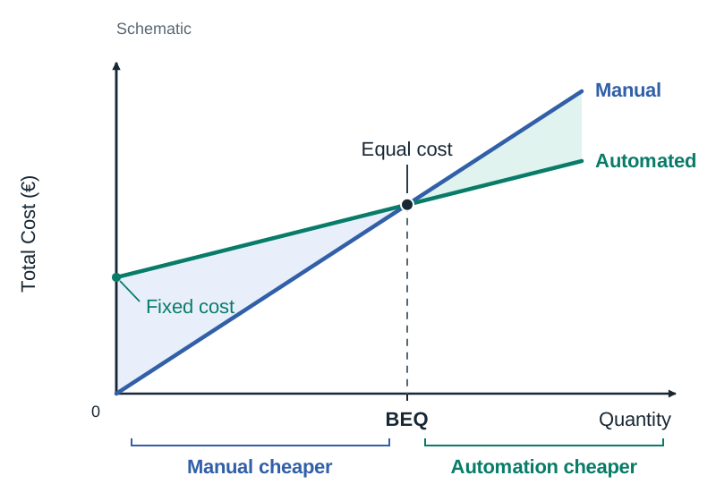
When choosing between two production methods—such as manual fabrication versus automated CNC tooling—engineers calculate the Break-Even Quantity (BEQ) where both options incur identical total costs:
- Volume below BEQ: Choose the option with the low fixed cost (manual or batch), because the order is too small to pay back the high cost of the tooling.
- Volume above BEQ: Choose the automated option; its higher fixed setup cost is amortised across the large batch, and its lower variable cost per unit yields substantial savings.
On a cost-volume graph, Total Cost (€) is plotted on the vertical axis and Quantity on the horizontal axis. A manual method with zero tooling starts at the origin and climbs steeply. An automated method starts at its fixed setup cost on the vertical axis and rises with a gentler slope. The intersection point marks the BEQ.
The Market Product Life Cycle and Concurrent Engineering
The Product Life Cycle (Sales against Time)
A commercial product progresses through four distinct market stages plotted on a curve of Sales against Time:
- Introduction: The product is launched. Sales are low and rise slowly because the market is unfamiliar with it. Heavy spending on advertising and tooling means little or no profit.
- Growth: The market accepts the product and sales rise rapidly. Unit costs fall as manufacturing volume increases, and competitors enter the market.
- Maturity: Sales reach their peak and level off. Competition is fiercest here, so manufacturers compete on price, quality, and cost reduction.
- Decline: Sales fall as the market becomes saturated or the product becomes technologically outdated.
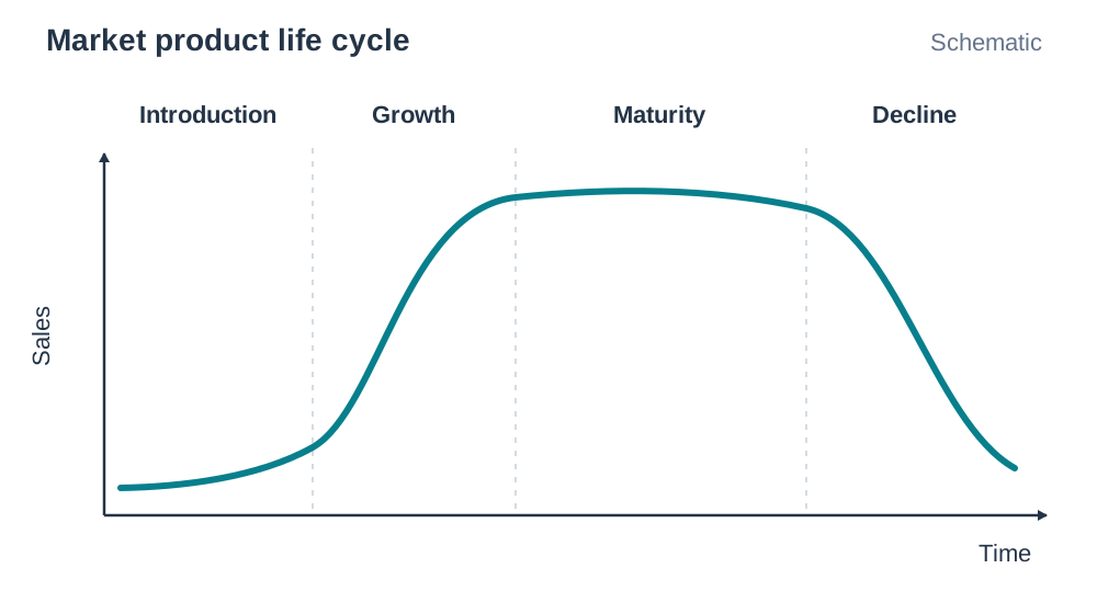
Extension Strategies are interventions applied during maturity to prolong the product's profitable life before it enters decline: restyling the casing, adding new features, offering fresh colour variants, targeting an export market, running a promotional campaign, or reducing the retail price.
Do not confuse the three course life cycles: the product life cycle (sales vs time), the reliability bathtub curve (failure rate vs operating hours), and the environmental life cycle (cradle-to-grave stages in DfE).
Concurrent Engineering and Design Teams
In traditional sequential ('over-the-wall') engineering, each department works in isolation. Designers hand drawings to production engineers, who discover manufacturing difficulties late, causing expensive tooling rework.
Concurrent Engineering replaces this sequence with parallel development managed by a cross-functional team (industrial designers, manufacturing engineers, procurement specialists, and quality technicians). Tooling, supply chains, and quality plans are developed simultaneously with the CAD model, dramatically reducing time to market and eliminating late engineering changes.
Market Research and the Product Design Specification (PDS)
Market research collects evidence to establish what the customer wants:
- Primary Research: Direct investigation (questionnaires, interviews, user observation, and prototype trials).
- Secondary Research: Existing published data (ISO/EN standards, competitor catalogues, CSO demographic tables).
A questionnaire should be short (8–10 questions), use closed tick boxes or 1–5 rating scales for easy quantification, avoid leading questions, and be piloted on a sample group before deployment. Findings are converted into a measurable Product Design Specification (PDS) with clear operational criteria: user anthropometrics, maximum allowable weight, operational voltage, target unit cost, and production batch size.
Quality Function Deployment (QFD) and Value Analysis
- Quality Function Deployment (QFD): A structured methodology using the House of Quality matrix to map customer requirements (Whats) against measurable engineering parameters (Hows). Weighting values quantify trade-offs and pinpoint technical priorities.
- Value Analysis (VA): Systematically interrogates an existing product to remove manufacturing costs without degrading performance, safety, or reliability:
The team evaluates every component: What does it do? Is this function essential? What does it cost? Can an alternative material or simpler geometry achieve the same function at lower cost? Should it be made in-house or purchased from a specialist supplier?
Design for Manufacture and Assembly (DFM/DFA) and CAD/CAM
Design for Manufacture and Assembly (DFM/DFA) reduces production cost and assembly time through practical engineering rules:
- Reduce the Part Count: Combine separate functions into a single injection moulding. Fewer components mean fewer manufacturing operations, lower inventory, and reduced assembly errors.
- Use Standard Components: Standard screws, bearings, and switches cost far less than custom parts and are immediately available from distributors.
- Design for the Forming Process: In plastic injection moulding, ensure uniform wall thicknesses to prevent sink marks, include generous draft angles (1° to 2°) to allow clean ejection from the mould, and use internal fillets to eliminate stress concentrations.
- Error-Proof the Assembly: Design parts to be symmetrical, or use asymmetric locating pins and chamfers so parts can only be assembled in the correct orientation (poka-yoke).
- Top-Down Assembly: Design components to stack vertically from a base plate so gravity assists assembly without rotating the product.
Role of 2D and 3D Parametric CAD
- 2D CAD: Used to generate dimensioned orthographic working drawings, sheet-metal flat patterns, and wiring schematics for fabrication.
- 3D Feature-Based (Parametric) CAD: Geometry is defined by dimensional constraints and editable features (extrude, revolve, fillet). Changing a single dimension updates the entire model, related assembly drawings, and CAM toolpaths automatically. It enables digital assembly interference checking, Finite Element Analysis (FEA) stress simulation, and direct export of STL/STEP files for 3D printing and CNC machining via G-codes.
Product Testing, Reliability, and Accelerated Testing
Product testing provides concrete evidence that a design performs safely, correctly, and reliably before volume production begins:
- Why Testing is Essential: Verifies that the product achieves its intended functions, ensures operator and user safety, confirms long-term durability, and detects flaws early when modifications are inexpensive.
- Categories of Testing:
- Function Testing: Confirms that the mechanism or circuit carries out its required task (e.g. verifying that an assistive pill dispenser releases exactly one dose).
- Safety Testing: Evaluates protection against electrical shock, sharp edges, excessive heat, and entrapment.
- Durability Testing: Assesses how well components withstand continuous wear, vibration, and environmental exposure.
- Destructive Testing: Tested on product samples to the point of mechanical failure to determine ultimate load limits and safety factors.
- Non-Destructive Testing (NDT): Inspects internal structure without damaging the part (e.g. ultrasonic or optical inspection for micro-cracks), leaving the item fully usable.
- The Reliability Bathtub Curve:
Product failure rate over operational lifetime follows a characteristic curve with three distinct phases:
- Infant Mortality (Early Failures): A high but rapidly decreasing failure rate caused by initial manufacturing flaws, poor soldering, or defective components. Interventions: Comprehensive burn-in testing before dispatch, stricter vendor inspection, and rigorous first-off checks.
- Useful Life (Random Failures): A low, steady, constant failure rate caused by unpredictable operational stresses. Interventions: Robust design safety margins and environmental protection.
- Wear-out Failures: An increasing failure rate as materials and parts reach the end of their operational lifespan through friction, fatigue, or aging. Interventions: Using higher-grade wear materials, designing modular parts for easy replacement, and scheduling preventive maintenance before wear-out begins.
- Accelerated Testing:
Testing a product's lifespan by running it under continuous, intensified operating conditions to compress years of normal service into days or weeks on an automated test rig. The total volume of operational use remains unchanged; only the timescale is compressed.
- Worked Calculation: An assistive living appliance is designed for a 10-year lifespan. Normal household usage is 3 cycles per week:
Running the appliance continuously on an automated test rig completes all 1,560 cycles in approximately two weeks, proving 10-year mechanical reliability before tooling funds are committed.
Design for Environment (DfE) and the Environmental Life Cycle
Design for Environment (DfE) is a structured design methodology that integrates ecological considerations into product development from the start, minimizing environmental harm across the entire product life cycle.
- The Five Environmental Life-Cycle Stages and Impacts:
- Raw Material Extraction: Mining ores, felling timber, or drilling petroleum for plastics depletes non-renewable finite resources and damages ecosystems.
- Manufacturing: Factory processing consumes electrical energy and water, generating machining scrap offcuts, chemical effluent, and emissions.
- Packaging and Transport: Burning fossil fuels in transit releases carbon emissions, while excess single-use packaging consumes material and generates waste.
- Use: Operating electrical appliances consumes energy over years (often the largest single environmental impact of the product's life cycle) and causes component wear.
- Disposal (End of Life): Discarded products sent to landfill consume ground space and risk toxic chemical leaching, while incineration releases atmospheric pollutants.
- Practical DfE Strategies:
- Material Selection: Minimise overall material mass, select renewable or recycled materials, and avoid toxic surface treatments or heavy metals.
- Cleaner Manufacturing: Nest component cut-outs to minimise sheet scrap, select low-energy forming processes, and recycle internal cutting fluids.
- Sustainable Packaging: Minimise packaging volume and specify unbleached, 100% recyclable mono-materials (e.g. corrugated cardboard) rather than bonded plastic-foil laminates.
- Energy-Efficient Use: Use low-power electronic components, energy-saving sleep modes, and high-efficiency motors to cut lifetime energy demands.
- Durability and Repair: Design modular products with easily accessible wear parts so products can be repaired rather than discarded.
- Design for Disassembly and Recycling: Use standard mechanical fasteners (screws, clips, snap-fits) rather than permanent adhesives or thermal welding; avoid bonding incompatible materials; and stamp universal polymer identification markings (ISO resin codes) directly on mouldings to allow rapid sorting at recycling centres.
- Coursework Application (2027 Thematic Brief: Ageing Society):
An assistive medication dispenser designed under DfE principles incorporates a single recyclable polymer housing (e.g. polypropylene) assembled with snap-fit joints and screws instead of adhesives, low-power circuitry, modular replacement drive gears, and unbleached cardboard packaging, ensuring full recyclability and easy repair.
(Note: Always distinguish this cradle-to-grave environmental life cycle from the market sales life cycle and the reliability bathtub curve.)
Quality Management: QC, QA, TQM, and Quality Plans
Quality represents conformance to customer requirements and technical specifications. Managing quality has progressed through three philosophies:
- Quality Control (QC) – 'Detect and Fix': A reactive method using end-of-line inspectors to check finished parts against drawings. Defective parts are scrapped or reworked. QC is inherently wasteful because materials, machine time, and labour have already been spent on the faulty item.
- Quality Assurance (QA) – 'Prevent and Build-in': A proactive system focusing on the production process. QA establishes standard operating procedures (SOPs), regular machine calibration, vendor audits, and poka-yoke (mistake-proofing) devices so faults are prevented during manufacture.
- Total Quality Management (TQM) – 'Company-Wide Culture': A holistic philosophy where quality is the responsibility of every employee, from directors to machine operators. It relies on worker empowerment, teamwork, and continuous incremental improvement (Kaizen).
TQM drives improvement using the Deming Cycle (PDCA):
- Plan: Identify process faults, map root causes, and design an experimental process adjustment.
- Do: Implement the proposed change on a controlled pilot production run.
- Check: Collect measurements to evaluate whether the defect rate dropped.
- Act: Standardise the new process parameters across the plant or adjust them if performance missed the target.
A Simple Quality Plan
A comprehensive quality plan outlines control points across the design and manufacturing stages:
- Design Stage: Establish measurable tolerances on CAD drawings, hold cross-functional design reviews, and test physical prototypes against the PDS.
- Incoming Inspection: Inspect bought-in materials and components using acceptance sampling before releasing them to production.
- First-Off Inspection: Inspect and measure the very first part produced after a machine setup or tool change. Full production cannot begin until this part is signed off.
- In-Process Checks: Operators check critical dimensions at regular intervals (e.g. every 20th part) using go/no-go gauges or micrometers, plotting results on control charts.
- Final Functional Test: Fully assembled items undergo 100% operational testing (e.g. electrical continuity, pressure containment, or switch actuation).
- Traceability and Quarantine: Defective parts are tagged, segregated in a quarantine bin, and logged for root-cause analysis.
Pareto Analysis and Problem-Solving (The 80/20 Rule)
The Pareto Principle states that roughly 80% of quality defects arise from approximately 20% of root causes. In quality problem-solving, a Pareto chart separates the 'vital few' problems from the 'trivial many':
- Constructing the Chart:
- Record defect occurrences and tally the frequency of each distinct defect type over an inspection run.
- Arrange defect categories in descending order of frequency from left to right along the horizontal axis.
- Draw vertical bars showing the count or cost of each defect type against the primary vertical axis.
- Plot an overlaid cumulative percentage curve (0% to 100%) against a secondary vertical axis on the right.
- Problem-Solving Application: Prioritise engineering interventions on the tallest bars on the far left. Eliminating these top one or two root causes removes the vast majority of overall defect costs.
- Worked Example: An inspection of 100 rejected moulded housings logs five defect types: flash (52), sink marks (28), surface scratches (10), warpage (6), and colour streaking (4). The first two categories account for 80% of all rejects (). By adjusting mould clamping force and cooling time to fix flash and sink marks, the engineering team eliminates 80% of scrap immediately without wasting time investigating the minor defects.
Statistical Process Control (SPC) and Control Charts
Every manufacturing process exhibits natural variation due to machine vibration, gear backlash, ambient temperature shifts, and minor metallurgical inconsistencies. A stable, normally distributed process is written as , where is the population mean and is the process standard deviation. Under this bell-shaped distribution, 68.27% of output falls within , 95.45% falls within , and 99.73% falls within , establishing a natural process spread of .
Constructing Control Charts
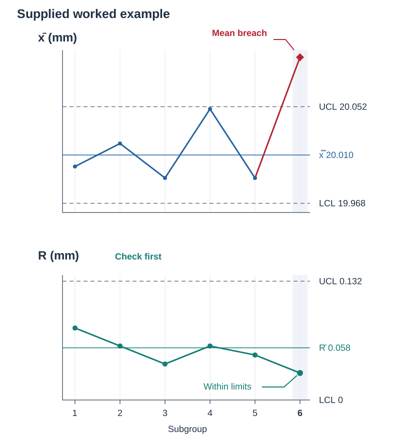
Statistical Process Control (SPC) tracks processes over time to identify assignable causes of error (such as worn bearings, chipped tool inserts, or operator fatigue) before out-of-specification scrap is produced. An system uses two linked charts constructed from subgroup samples of size (typically or consecutive items) taken at regular intervals:
- Chart (Mean Chart): Monitors the central tendency of the process to detect drift in the mean setting.
- Chart (Range Chart): Monitors process spread and consistency by tracking the sample range ().
Control limits are calculated from the grand mean () and average range ():
| Subgroup Sample Size () | ||||
|---|---|---|---|---|
| 4 | 0.729 | 0 | 2.282 | 2.059 |
| 5 | 0.577 | 0 | 2.114 | 2.326 |
Interpreting the Charts
A process is out of control if any plotted sample point breaches the Upper Control Limit (UCL) or Lower Control Limit (LCL), or if non-random patterns appear, such as seven consecutive points resting on one side of the centreline or a continuous upward run indicating gradual tool wear. Always evaluate the chart first; if variation is out of control, mean control limits become mathematically invalid.
Process Capability Indices and Component Acceptance Sampling
Control charts verify whether a process is stable; process capability indices determine whether a stable process can manufacture parts inside the customer's design tolerances.
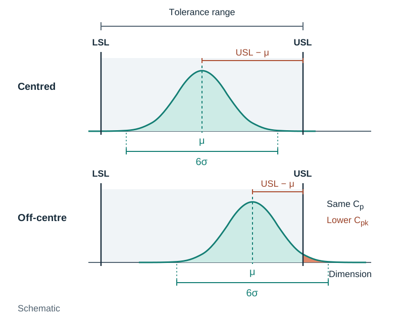
- Upper Specification Limit (USL) & Lower Specification Limit (LSL): The maximum and minimum dimensions permitted by the engineering drawing.
- Tolerance Range: .
Capability Indices: and
(Potential Capability): Measures whether the machine's natural variation () fits inside the permitted tolerance band, assuming the process is centred:
- : The process is capable. Natural spread is narrower than the customer's tolerance window.
- : The process is marginally capable. The spread matches the tolerance window, resulting in an expected 0.27% defect rate if centred.
- : The process is not capable. Natural machine variation will inevitably produce non-conforming scrap.
(Actual Capability): Evaluates capability while accounting for process off-centring relative to specification boundaries:
If is high but , the process has adequate precision but is improperly centred, requiring tool adjustment rather than machine replacement.
Component Sampling Inspection Plans
Inspecting 100% of received parts is slow, expensive, and subject to human inspector fatigue; it is also impossible for destructive testing (e.g. tensile breaking tests). Manufacturers use statistical acceptance sampling where a representative sample size () is drawn at random from a delivery batch of size :
- Acceptable Quality Level (AQL): The worst average defect rate that the customer considers acceptable.
- Acceptance Number (): The maximum number of defective parts allowable in the sample. If defects , the batch is accepted; if defects , the batch is rejected.
- When a contractual sampling percentage () is specified, calculate sample size using and always round up to the nearest integer. If the exam question provides an inspection table or sampling scheme, read directly from the plan.
- Sampling Risks: Producer's Risk is the probability of rejecting an acceptable batch due to bad luck in the sample; Consumer's Risk is the probability of accepting a substandard batch.
Just-in-Time (JIT) Manufacturing, Seven Wastes, and Kanban Systems
Traditional manufacturing operates as a push system, where large batches are produced against forecasts and stored as inventory. Holding inventory ties up capital, requires warehouses, risks product obsolescence, and hides problems like machine breakdowns or supplier delays.
Just-in-Time (JIT) is a lean pull system where materials arrive and products are made only as required by the next downstream operation. JIT aims to eliminate the seven wastes (remember TIMWOOD):
- Transport: Moving parts further than necessary. JIT positions supplying machines adjacent to consuming stations.
- Inventory: Raw stock, work-in-progress, and finished goods sitting idle. JIT holds only what is needed immediately, freeing cash and floor space.
- Motion: Unnecessary operator bending, stretching, or walking. Solved by ergonomic, U-shaped cell layouts.
- Waiting: Operators or machines idle due to late deliveries or upstream bottlenecks. Balanced cycle times reduce waiting.
- Over-production: Producing more or earlier than the customer requires. In JIT, nothing is made without a Kanban authorization.
- Over-processing: Doing more work than specified (e.g. polishing a non-visible surface or holding unnecessarily tight tolerances).
- Defects: Scrap and rework. Because there is no buffer stock, defects stop the line, forcing immediate root-cause correction at source.
Kanban Loop Mechanics and Sizing
Kanban (meaning 'sign' or 'card') is the visual control mechanism that runs a JIT pull system. Upstream workstations are forbidden from producing parts until an empty container or Kanban card arrives from downstream, pulling parts through the plant strictly in response to real consumption.
- : Demand rate (units required per hour).
- : Replenishment lead time (hours).
- : Safety stock allowance factor (decimal, e.g. 0.15 for 15%).
- : Container capacity (parts per bin).
- Remember to round up so the cell is never starved of parts.
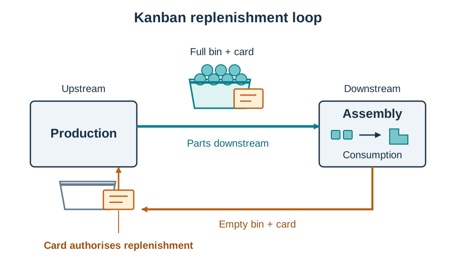
In lean manufacturing, managers intentionally remove a Kanban card from the loop to lower stock levels. This exposes the next bottleneck—such as a slow machine changeover or unreliable tool—allowing the team to fix it. This is how JIT drives continuous improvement (Kaizen).
Measuring Manufacturing Performance
The syllabus requires you to describe and measure performance:
- Throughput Rate: Units produced divided by operating hours. A cell producing 300 units over a 7.5-hour shift has a throughput of .
- Manufacturing Lead Time: The total elapsed time from raw material release to final packing (e.g. released at 09:00, packed at 11:15 = 2.25 hours).
- Defect Rate: . If 12 of 300 units are rejected, .
- Machine Utilisation: .
Project Management: Team Dynamics and Behavioural Factors
Complex manufacturing projects require effective team collaboration. A cross-functional team outperforms individuals by combining diverse technical skills, sharing the workload, and reviewing designs before tooling funds are committed.
Common Team Roles: Coordinator/Leader (monitors the schedule), Ideas Person/Designer (generates concepts), Technical Specialist/Maker (evaluates fabrication), Quality/Test Specialist (validates tolerances), and Recorder (documents minutes and drawings).
Stages of Team Development (Tuckman):
- Forming: Members meet, explore the project brief, and identify initial goals. Roles and responsibilities remain tentative.
- Storming: Conflict arises as members argue over design concepts, project leadership, and workload distribution. This is the most difficult stage.
- Norming: The team resolves differences, agrees on ground rules, establishes clear working roles, and commits to a single design direction.
- Performing: The team operates smoothly and autonomously to achieve project milestones, resolving technical problems through evidence.
Behavioural Factors in TQM: Total Quality Management succeeds through people, not just statistical charts. Operators must be trained in problem-solving techniques, empowered to stop the line when a defect occurs (an Andon cord system), organised into quality circles to suggest process improvements, and provided with transparent defect data feedback.
Work Cell Design, Ergonomics, Safety Legislation, and Simulation
Designing the Work Cell around the Operator
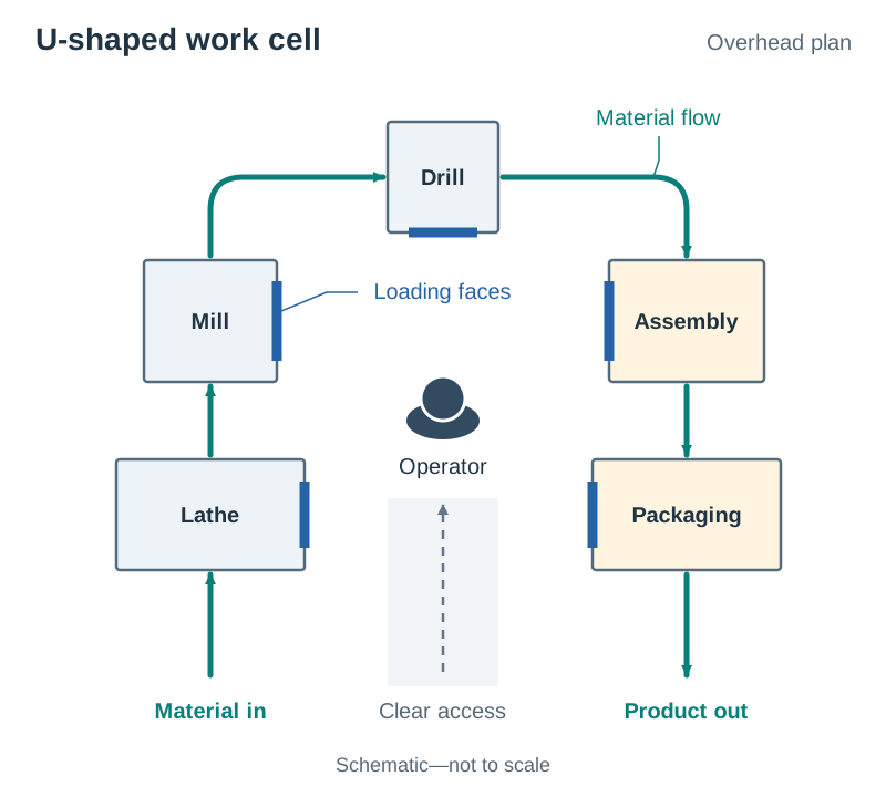
A work cell groups dissimilar machines together to complete the manufacture of a family of related components. Cells are typically arranged in a U-shape so the start and end of the line are close together, allowing one operator to manage multiple machines and reducing walking distances.
Work cell design must accommodate three major constraints:
- Human Factors (Ergonomics): Workstations must be dimensioned to anthropometric data. Light assembly work surfaces are positioned at elbow height (roughly 900–1000 mm for standing work). Workpieces, tools, and bins must sit within the normal reach envelope (400–500 mm). Provide anti-fatigue floor matting, adjustable seating with lumbar support, adequate task lighting (minimum 500 lux), and task rotation to prevent Repetitive Strain Injury (RSI).
- Health and Safety Legislation: The Safety, Health and Welfare at Work Act 2005 places a statutory duty on employers to provide a safe place of work, safe machinery, and safe systems of work. Employers must conduct formal risk assessments and prepare a written Safety Statement. Machine tools must feature fixed interlocking guards and emergency stop buttons within immediate reach of every station. The Health and Safety Authority (HSA) inspects facilities and enforces statutory compliance.
- Workflow Constraints: Material enters at one end of the cell and moves smoothly to the exit without crossing paths or backtracking. Aisles must be wide enough for component trolleys and kept clear of work-in-progress.
Principles of Plant Layout
Plant layout is the strategic arrangement of machines, equipment, and workstations to ensure efficient workflow:
- Process Layout (Functional Layout): Machines performing similar operations are grouped together into dedicated departments (e.g. all lathes in one shop, all milling machines in another). Ideal for job and batch production where product variety is high. Highly flexible, but parts travel long, complex routes through the facility, resulting in high material handling costs and large work-in-progress inventory.
- Product Layout (Flow Line / Assembly Line): Machines and workstations are arranged strictly in the sequential order required to manufacture a single product. Ideal for high-volume mass production of standardised items. Highly efficient with minimal transit times, but completely inflexible to design changes and vulnerable to whole-line stoppages if one station breaks down.
- Cellular Layout (Work Cells): Dissimilar machines are grouped into dedicated, self-contained cells (often arranged in a U-shape) to produce a family of related components. It combines the flexibility of a process layout with the smooth, rapid flow of a product layout.
Capacity Management and Strategic Planning
Capacity is the maximum rate of output a manufacturing facility or production line can achieve over a defined timeframe (e.g. units per week).
- Capacity Strategies:
- Lead Strategy: Expanding production capacity before customer demand increases. Advantage: Guarantees meeting market surges and captures market share. Risk: High capital expenditure and expensive idle overheads if sales forecasts fail to materialise.
- Lag Strategy: Expanding capacity only after demand has already increased and proven sustainable. Advantage: Minimises financial risk and avoids paying for unused equipment. Risk: Production cannot meet peak demand, leading to lost sales, extended lead times, and dissatisfied customers.
- Average (Match) Strategy: Adding capacity incrementally to track average demand forecasts. Advantage: Moderates the financial risks of excess idle capacity while limiting lost orders.
- Optimum Capacity Level: The production volume where manufacturing cost per unit reaches its lowest point. Operating well below optimum spreads fixed factory overheads over too few units, increasing unit cost; operating continuously at 100% capacity overstrains machinery, leading to frequent breakdowns and quality errors.
- Capacity Cushion: A planned reserve margin (typically 10%–20% above expected demand) kept to absorb sudden demand spikes, preventive maintenance, or delivery delays without interrupting supply.
Flow-Line Scheduling and Line Balancing
Activity scheduling organizes the sequence and timing of manufacturing operations to meet customer delivery dates efficiently.
- Cycle Time (): The target time interval between consecutive completed products emerging from the end of the line:
- Theoretical Minimum Workstations (): The fewest workstations needed to complete all tasks within the required cycle time:
- Line Balancing Efficiency: Measures how evenly assembly work is distributed across stations, minimising idle waiting time:
- Worked Example (Flow Line Scheduling):
A flow line has 480 minutes available per shift to produce 160 units. The sum of all individual assembly task times is 9.0 minutes.
- Step 1 — Calculate Cycle Time:
- Step 2 — Determine Minimum Workstations:
- Step 3 — Calculate Line Efficiency if 4 stations are actually used:
Production Planning: Gantt Charts and the Critical Path Method (CPM)
- Gantt Chart: A visual project planning tool plotting scheduled tasks as horizontal bars against a calendar timeline. It shows task start dates, durations, dependencies, and milestones, enabling project managers to compare planned schedules against actual progress.
- Critical Path Method (CPM): A network scheduling technique that identifies task dependencies. The Critical Path is the longest unbroken sequence of dependent activities from project start to finish. It determines the shortest possible project completion time. Tasks on the critical path have zero float—any delay to a critical activity delays the entire project completion date.
- Float (Slack Time): The duration an activity can slip without delaying the final project deadline:
Simulation Tools and Simulation Games
- Discrete-Event Simulation Software: Digital models of a manufacturing cell or factory layout. Users input processing times, machine breakdown rates, changeover times, and part arrival rates. The software runs thousands of cycles to reveal bottlenecks, predict average lead times, calculate machine utilisation, and test layout modifications without spending capital.
- Spaghetti (String) Diagrams: A physical or digital mapping tool that traces the exact walking path of an operator or the movement of a component over a factory floor drawing. A tangled diagram indicates wasted transport and motion.
- Simulation Games: Hands-on classroom exercises comparing push production (producing to forecast, resulting in massive work-in-progress piles) against pull production (Kanban authorization, resulting in smooth, balanced flow).
Key terms
- Added Value
- The increase in worth given to raw materials through manufacturing operations, calculated as the market selling price minus the raw material and resource costs.
- Product-Process Matrix
- A strategic framework matching product volume and variety to the appropriate manufacturing method: Job, Batch, Mass, or Continuous.
- Break-Even Quantity (BEQ)
- The exact production volume at which the total costs of two alternative manufacturing methods (or total costs and total revenues) are equal.
- Total Quality Management (TQM)
- A company-wide management culture where all employees continuously improve processes and product quality to achieve customer satisfaction.
- Pareto Principle
- The observation that roughly 80% of quality defects arise from approximately 20% of root causes, evaluated using a descending bar chart with an overlaid cumulative percentage line.
- x-R Control Chart
- A pair of Statistical Process Control charts tracking subgroup averages (x-bar) to monitor the process mean, and subgroup ranges (R) to monitor process spread against calculated limits.
- Process Capability Index (Cp)
- A statistical ratio comparing the design tolerance range (USL - LSL) to the natural variation spread (6-sigma) of a stable manufacturing process.
- Cpk
- A capability index that evaluates how close a process is operating to its nearest specification limit, taking process off-centring into account.
- Just-in-Time (JIT)
- A lean production philosophy where parts arrive and products are manufactured only when triggered by downstream demand, eliminating warehouse buffer inventory.
- Kanban
- A visual card, container, or electronic signal that controls production in a pull system by authorising an upstream station to produce a set quantity of parts.
- Concurrent Engineering
- A product development approach where cross-functional teams work in parallel from the beginning, considering design, tooling, assembly, and maintenance concurrently.
- Quality Function Deployment (QFD)
- A structured methodology using the House of Quality matrix to translate customer requirements (the Voice of the Customer) into quantifiable engineering specifications.
- Value Analysis
- A systematic review of a product's components to eliminate unnecessary manufacturing costs while maintaining or improving necessary function, safety, and quality.
- Design for Manufacture and Assembly (DFM/DFA)
- A design methodology focused on reducing part counts, standardising components, and creating error-proof geometry to make manufacturing and assembly simple and economical.
- Work Cell
- A dedicated, self-contained layout of different machines arranged in sequence (typically a U-shape) to complete the manufacture of a family of parts.
- Bathtub Curve
- A failure-rate curve over operational time showing three lifecycle phases: infant mortality (decreasing), useful life (constant), and wear-out (increasing).
- Cycle Time
- In flow production, the target time interval between consecutive completed units leaving the end of the production line.
- Design for Environment (DfE)
- A design methodology integrating ecological considerations across the entire product life cycle to minimise resource consumption, emissions, and waste.
Check yourself
Name the four stages of the market product life cycle and give two extension strategies.
Introduction, Growth, Maturity, and Decline. Extension strategies: adding new features or colours, updating styling, entering export markets, changing packaging, or reducing price.
Name any four of the seven wastes in lean manufacturing and state how JIT reduces one of them.
Transport, Inventory, Motion, Waiting, Over-production, Over-processing, and Defects (TIMWOOD). Example: JIT eliminates over-production by requiring a Kanban pull signal before any parts are manufactured.
A production run of 200 brackets has direct material costs of €330, direct labour of €900, and allocated overheads of €480. Find the unit cost and the selling price with a 25% profit mark-up.
Total cost = 330 + 900 + 480 = €1,710. Unit cost = 1,710 / 200 = €8.55 per bracket. Selling price = 8.55 * 1.25 = €10.69 per bracket.
State two ergonomic and two health and safety legal requirements to consider when designing a manufacturing work cell.
Ergonomic: set bench height to anthropometric elbow height (900–1000 mm for standing), keep tools inside normal reach envelope (400–500 mm). Legal: provide interlocking machine guards, carry out risk assessments / Safety Statement under the Safety, Health and Welfare at Work Act 2005.
What is the difference between an Order Qualifier and an Order Winner?
An Order Qualifier is a baseline standard required just to be considered by customers (e.g. CE mark); an Order Winner is the decisive factor that wins the sale (e.g. lowest price or fastest delivery).
A flow line has 480 minutes available per shift to produce 160 units. Total task time is 9 minutes. Find the cycle time, minimum workstations, and the line balancing efficiency if 4 workstations are actually used.
Cycle time = 480 / 160 = 3 minutes. Minimum workstations = 9 / 3 = 3 stations. Line efficiency = [9 / (4 3)] 100 = 75% (with 25% balance delay).