Statistics - Descriptive Statistics

1. Data Gathering and Study Design

Calculations mean nothing if your data collection is flawed from the start. Statistical data can be categorical (nominal with no natural order, or ordinal with a defined order) or numerical (discrete when counted, or continuous when measured). A sample survey collects data from a subset of a population to make inferences about the entire group. In an observational study, researchers record natural behaviors or outcomes without intervening or altering any conditions. A designed experiment deliberately imposes a specific treatment on subjects to observe its effect. Crucially, only a randomised designed experiment featuring an appropriate control group can demonstrate direct cause and effect.

You must also understand four core sampling strategies:

• Simple Random Sampling: Every member of the population has an equal probability of selection.
• Stratified Sampling: The population is divided into non-overlapping groups (strata), and random samples are drawn proportionally from each stratum.
• Cluster Sampling: The population is divided into clusters, and entire clusters are chosen at random to be surveyed.
• Quota Sampling: Non-random sampling where interviewers select participants until specified category quotas are filled.

Be ready to evaluate statistical bias. Selection bias arises when certain demographics are systematically excluded from the sampling frame. Non-response bias occurs when individuals who decline to participate differ substantially in character from those who do. Identifying these biases explicitly earns full marks on experimental design questions.

2. Measures of Centre and Spread

For numerical data, your primary measures of central tendency are the mean and the median. For grouped frequency distributions where individual scores are unknown, we estimate the mean by finding the mid-interval value ($x$) and applying the formula:

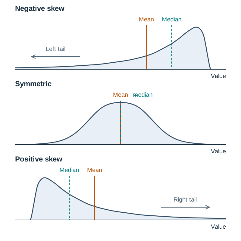
The median ($Q_2$) represents the exact middle observation once values are ranked in order. When a distribution is symmetric, the mean and median lie very close together. In a positively skewed distribution with a long right tail, high values pull the mean above the median. In a negatively skewed distribution with a long left tail, low values pull the mean below the median.

Measures of dispersion reveal how data spreads around the centre. To find quartiles, first rank the data in ascending order and find the median ($Q_2$); the lower quartile ($Q_1$) is the median of the values below $Q_2$, and the upper quartile ($Q_3$) is the median of the values above $Q_2$. More broadly, the $p^{\text{th}}$ percentile ($P_p$) is the value below which $p\%$ of the ranked data lie, so $Q_1 = P_{25}$, the median = $P_{50}$, and $Q_3 = P_{75}$. Saying a student is at the $90^{\text{th}}$ percentile describes position in the group (90% scored at or below that value), not a percentage mark of 90%. The interquartile range (IQR) measures the spread of the central 50% of ordered observations: $\text{IQR} = Q_3 - Q_1$. A data point is formally classified as an outlier if it satisfies either of the following conditions:

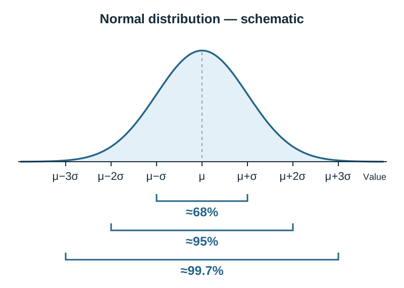
Because outliers heavily distort the mean and standard deviation, you should always report the median and IQR for skewed data or distributions with outliers. For symmetric distributions without extreme values, the standard deviation ($\sigma$) is preferred: $\sigma = \sqrt{\frac{\sum (x - \bar{x})^2}{n}}$. To calculate it, square each value's distance from the mean, average these squared distances, and take the square root; the answer is in the same units as the data, and $\sigma^2$ is called the variance. In practice, you normally read this value directly from your calculator: always select the population standard deviation $\sigma_x$, which matches the formula on page 33 of your Formulae and Tables booklet, rather than the sample statistic $s_x$. Furthermore, many measurements form a symmetric, bell-shaped (normal) distribution. For normally distributed data, the empirical rule states that approximately 68% of values lie in $[\mu - \sigma, \mu + \sigma]$, 95% lie in $[\mu - 2\sigma, \mu + 2\sigma]$, and 99.7% lie in $[\mu - 3\sigma, \mu + 3\sigma]$. For example, if bags of crisps have $\mu = 50\text{ g}$ and $\sigma = 2\text{ g}$, a weight of $54\text{ g}$ is $\mu + 2\sigma$, so about 5% lie outside $\pm 2\sigma$, and by symmetry about 2.5% exceed $54\text{ g}$ (about 100 bags in 4000). Remember that these percentages apply only when the question states the data is normally distributed; use the median and IQR if it is skewed.

3. Graphical Displays and Bivariate Data

Choosing an effective graphical display depends directly on the structure of your data. A stem-and-leaf plot is ideal for small to medium univariate numerical datasets because it preserves raw values while ordering the distribution. Every stem-and-leaf plot needs a precise key (for example, $4 \mid 2 = 42\text{ marks}$) — without it the numbers cannot be read, so always include one. For continuous data grouped into intervals, use a histogram where adjacent bars touch. To compare two distributions side by side, draw back-to-back stem-and-leaf plots or box plots sharing an identical continuous scale.

When exploring the relationship between two numerical variables recorded for the same subjects, use bivariate data plotted on a scatterplot. Place the independent or explanatory variable on the horizontal $x$-axis and the dependent or response variable on the vertical $y$-axis. The correlation coefficient ($r$) quantifies the direction and strength of the linear relationship on a scale from $-1$ to $+1$:

• $r = +1$: Perfect positive linear correlation
• $r = 0$: No linear relationship
• $r = -1$: Perfect negative linear correlation

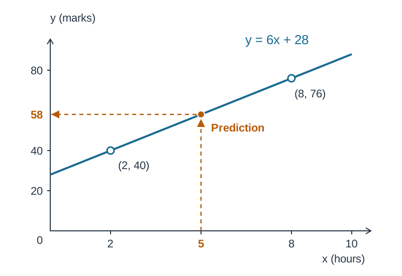
You can compute $r$ directly using your calculator's bivariate statistics menu ($A + Bx$ mode). You should also be able to draw a line of best fit by eye on a scatterplot so that it follows the linear trend with roughly as many points above as below, ideally passing through the mean point $(\bar{x}, \bar{y})$. You can read predicted values directly from the line or find its equation using two points on it with $y - y_1 = m(x - x_1)$. For example, a line through $(2, 40)$ and $(8, 76)$ has slope $m = \frac{76 - 40}{8 - 2} = 6$ and equation $y - 40 = 6(x - 2) \implies y = 6x + 28$; for $x = 5\text{ hours}$, it predicts $y = 6(5) + 28 = 58\text{ marks}$. Remember that predictions far outside the range of the data (extrapolation) are unreliable. Always remember: correlation does not imply causality. A strong linear relationship between two variables may be coincidental or driven by an unobserved lurking variable.

Key terms

Outlier

A data value that lies more than 1.5 times the interquartile range below Q1 or above Q3: outside [Q1 - 1.5(IQR), Q3 + 1.5(IQR)].

Standard Deviation

A measure of spread found by averaging the squared distances of the values from the mean and taking the square root: $\sigma = \sqrt{\frac{\sum (x - \bar{x})^2}{n}}$. The square of the standard deviation, $\sigma^2$, is called the variance.

Mid-interval Value

The midpoint of a class interval, obtained by averaging its lower and upper boundaries, used to approximate the mean in grouped data.

Skewness

The asymmetry of a data distribution; a positive skew features a long tail to the right (mean > median), while a negative skew features a long tail to the left (mean < median).

Correlation Coefficient (r)

A statistical value between -1 and +1 that measures the strength and direction of the linear relationship between two variables.