The Labour Market

1. Factor Markets and Derived Labour Demand

In a goods and services market, households act as the buyers (consumers) and firms act as the sellers of final products like groceries or haircuts. In a factor market, these roles are reversed. Households are the sellers, supplying their labour, land, or capital, while firms are the buyers, purchasing inputs to produce output. The price paid in the labour market is a factor reward: the wage.

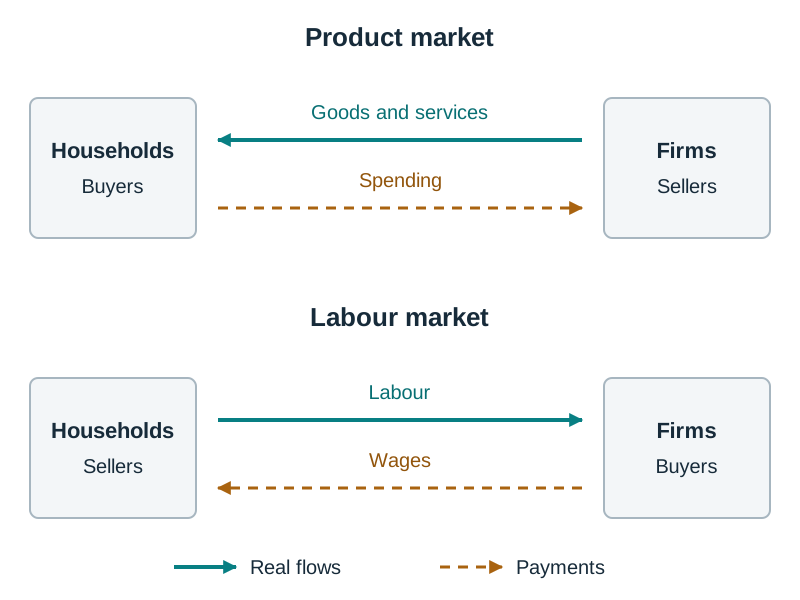
The four factors of production and their rewards are:

• Land: All natural physical resources (farmland, mineral deposits, water). Its factor reward is Rent.
• Labour: All human physical and mental effort used in production. Its factor reward is Wages.
• Capital: Goods made by people that are used to produce other goods and services, such as machinery, tools, and factories. Its factor reward is Interest.
• Enterprise: The managerial initiative to combine the other three factors and assume commercial risk. Its factor reward is Profit.

Firms do not hire staff for personal consumption. Demand for labour is a derived demand, meaning it depends directly on consumer demand for the final goods or services those workers produce. If consumer demand for airline travel drops, airlines need fewer flights, so their demand for pilots, cabin crew, and ground staff decreases.

Movements along versus shifts of the demand curve

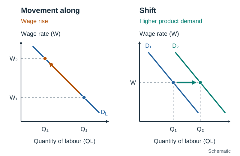
A change in the wage rate causes a movement along the existing labour demand curve. When wages rise, the quantity of labour demanded contracts; when wages fall, it expands. By contrast, non-wage factors shift the entire labour demand curve:

• Consumer demand for the final product: Higher demand for goods shifts the labour demand curve to the right as firms hire to boost output.
• Worker productivity: When staff produce more output per hour through better skills or technology, their higher productivity shifts labour demand to the right.
• Relative price of capital: If automated checkouts or machinery become cheaper relative to wages, firms replace workers with capital, shifting the labour demand curve to the left.
• Non-wage labour costs: An increase in employer Pay-Related Social Insurance (PRSI) raises the total cost of each worker, shifting labour demand to the left.

The market demand curve for labour slopes downward from left to right. This downward slope reflects the law of diminishing returns: because capital is fixed in the short run, adding successive units of variable labour eventually causes each additional worker to add less extra output than the worker before them.

2. Marginal Productivity Theory: MPP and MRP

To determine how many workers to employ, a profit-maximising firm calculates marginal productivity.

• Marginal Physical Product (MPP): The extra physical output produced by employing one additional unit of labour, keeping all other factor inputs constant:

• Marginal Revenue (MR): The extra revenue gained from selling one more unit of output.

• Marginal Revenue Product (MRP): The additional revenue a firm earns from selling the output produced by employing one extra worker:

Under perfect competition in the product market, the firm is a price taker, so MR equals the market price ($P$). Therefore, $\text{MRP} = \text{MPP} \times P$. Under imperfect competition, the firm faces a downward-sloping demand curve and must drop its price to sell more units. Because MR falls as output expands (MR < P), the firm's MRP curve slopes downward more steeply.

The profit-maximising hiring rule

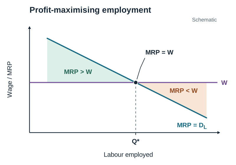
In a competitive labour market, a firm maximises profit by hiring workers up to the point where Marginal Revenue Product equals the wage rate:

• When $\text{MRP} > W$, the worker brings in more extra revenue than they cost in wages, adding to total profit.
• When $\text{MRP} < W$, the worker costs more than they add to revenue, reducing total profit.
• With table data where workers are added in whole numbers, keep hiring each extra worker as long as their MRP is greater than or equal to the wage ($\text{MRP} \ge W$). Stop before the first worker whose MRP falls below the wage.
• Because a firm hires up to the point where MRP equals the wage, the downward-sloping segment of the MRP curve acts as the firm's demand curve for labour.

Usefulness to employers

• Deciding employment levels: It provides a precise mathematical cut-off: hiring stops where $\text{MRP} = W$.
• Setting the maximum wage: A worker's MRP is the upper limit of what an employer can pay them without making a loss on their employment.
• Evaluating capital and training investments: If funding staff upskilling or new equipment lifts MPP and MRP by more than the cost of the investment, the spending is profitable.
• Responding to price changes: If final product prices drop, MR and MRP fall immediately, warning the business that it must reduce staff numbers or cut wage costs.

Usefulness to employees and trade unions

• Backing wage claims: Demonstrating that worker training or technology has increased MPP provides measurable evidence to justify pay rises during collective bargaining.
• Assessing job security: Workers whose MRP exceeds their wage are profitable and secure; workers whose MRP falls below the market wage face risk of redundancy.
• Guiding career development: Workers can see that learning scarce skills raises their MPP and MRP, directly boosting their long-term earning power.

Limitations of marginal productivity theory

• Measuring output in service jobs: In public and service sectors—such as nursing, policing, or teaching—output cannot be counted in physical units or sold at a market price, making MRP impossible to calculate directly.
• Team production: In modern firms, goods and services are produced collaboratively. Isolating the exact individual output of one software engineer or assembly technician is rarely practical.
• Wages set outside the market: Pay rates are often fixed by national public-sector pay deals, trade union agreements, or statutory minimum wage rates rather than individual MRP.
• Other factors do not stay fixed: The theory assumes capital, tools, and technology stay constant when an extra worker arrives, but in reality extra staff often require additional machinery or workspace.

3. The Supply of Labour and Market Equilibrium

The supply of labour represents the number of hours of work individuals are willing and able to offer at any given wage rate.

Determinants of labour supply

• The wage rate: Higher wages increase the financial return from working, drawing more people into an industry or motivating longer hours.
• The participation rate: This is the percentage of the working-age population (aged 15–64) that is in the labour force, either working or looking for work. A rise in participation expands total labour supply.
• Childcare costs and availability: High childcare costs act as a financial barrier to work. State supports, such as Ireland's National Childcare Scheme (NCS), lower this barrier and increase the supply of available labour, particularly among parents.
• Retirement age and pensions: Raising the statutory pension age or modifying occupational pension rules keeps older workers in the workforce longer, increasing labour supply.
• Numbers in full-time education: As more school leavers attend third-level colleges and training programmes, the supply of young labour drops in the short run, though it builds a more qualified workforce over time.
• Working conditions and non-monetary rewards: Job security, flexible hours, subsidised pensions, and generous annual leave encourage people to take up work even where the basic pay is modest.
• Net migration: Inward migration expands the workforce by filling shortages in sectors such as construction, IT, and healthcare. Outward migration during economic downturns contracts domestic labour supply.
• Taxes and social welfare: High marginal income taxes cut take-home pay, while generous social welfare supports can create an unemployment trap where the net financial gain from working is too small to incentivise taking a job.

The individual backward-bending supply curve

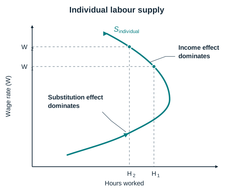
While the market supply curve for an entire occupation slopes upward from left to right, an individual person's supply curve can bend backward at high wages because of two competing influences:

1. The substitution effect: As the wage rises, the opportunity cost of leisure increases because taking time off means sacrificing more pay. The worker substitutes work for leisure, offering more hours.
2. The income effect: As the wage climbs higher, the worker earns enough to afford their desired standard of living in fewer hours. Because leisure is a normal good, their demand for free time rises, so they choose to work fewer hours.

At low and moderate wages, the substitution effect outweighs the income effect, making the supply curve slope upward. Beyond a critical wage threshold, the income effect overpowers the substitution effect, causing the individual supply curve to bend backward toward the vertical axis.

Equilibrium wage determination

In a free, unregulated labour market, the equilibrium wage ($W_e$) and equilibrium quantity of labour ($Q_e$) sit where the market demand curve ($D_L$) crosses the market supply curve ($S_L$). At $W_e$, the number of workers businesses wish to employ matches the number of workers willing to work.

4. Government Interventions: Minimum Wage, Taxation, and Regulation

Governments intervene in labour markets to protect workers' living standards, collect public revenue, and correct market failures.

The National Minimum Wage

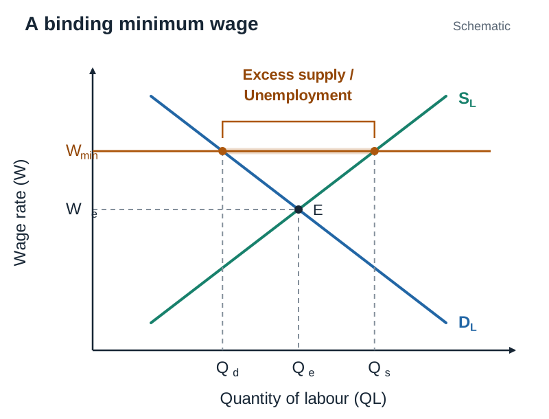
The National Minimum Wage acts as a legal price floor. In Ireland, it rose to €14.15 per hour from January 2026, with the government committed to moving toward a living wage set at 60% of median hourly earnings. (Always verify the prevailing rate when preparing for the examination.) When set above the free-market equilibrium wage ($W_e$):

• At the higher wage, the quantity of labour supplied expands to $Q_s$ because more people are drawn into the job market.
• The quantity of labour demanded by firms contracts to $Q_d$ as employers economise on higher payroll costs.
• The difference between $Q_s$ and $Q_d$ is an excess supply of labour, which is unemployment.
• Economic trade-offs: Low-paid workers who keep their jobs enjoy higher disposable income, reducing in-work poverty and lifting consumer spending. On the other hand, employers face higher operating costs, which can cause possible job losses in labour-intensive firms such as hospitality and retail, reductions in working hours, or higher retail prices passed to consumers (cost-push inflation).

How to draw the minimum wage diagram

1. Draw a vertical axis labelled 'Wage Rate (W)' and a horizontal axis labelled 'Quantity of Labour (QL)'.
2. Draw a downward-sloping labour demand curve ($D_L$) and an upward-sloping labour supply curve ($S_L$).
3. Mark their intersection at equilibrium wage $W_e$ and equilibrium employment $Q_e$.
4. Draw a horizontal line across the graph strictly above $W_e$ and label it '$W_{\text{min}}$' (or 'NMW').
5. Where this horizontal line cuts $D_L$, drop a vertical dashed line to the horizontal axis and label it '$Q_d$'.
6. Where this line cuts $S_L$, drop a vertical dashed line to the horizontal axis and label it '$Q_s$'.
7. Clearly label the horizontal gap between $Q_d$ and $Q_s$ as 'Excess Supply / Unemployment'.

How to draw the labour taxation diagrams

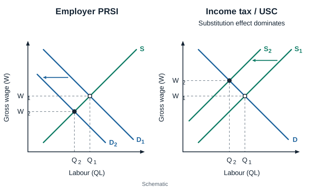
Effect of an increase in Employer PRSI (a tax on hiring):

1. Use axes labelled 'Wage Rate (W)' and 'Quantity of Labour (QL)'.
2. Draw the original downward-sloping demand curve $D_1$ and upward-sloping supply curve $S$. Mark equilibrium at $W_1$ and $Q_1$.
3. Draw a new demand curve $D_2$ parallel and to the left of $D_1$. Because each employee now costs more than their wage in mandatory payroll taxes, firms demand fewer workers at every wage level.
4. Mark the new intersection where $D_2$ crosses $S$ at a lower market wage $W_2$ and a lower employment level $Q_2$.
5. Explain: Employer PRSI raises hiring costs, shifting labour demand left, which cuts equilibrium employment from $Q_1$ to $Q_2$ and depresses the wage received by workers.

Effect of an increase in Income Tax or USC (a tax on employees):

1. Use axes labelled 'Wage Rate (W)' and 'Quantity of Labour (QL)'.
2. Draw original curves $D$ and $S_1$, marking equilibrium at gross wage $W_1$ and employment $Q_1$.
3. Draw a new supply curve $S_2$ parallel and to the left of $S_1$. Higher income tax cuts net take-home pay at every gross wage, reducing the incentive to work overtime or take up jobs.
4. Mark the new equilibrium where $S_2$ crosses $D$ at a higher gross wage $W_2$ and lower employment $Q_2$.
5. Explain: A tax on earnings shifts labour supply left, forcing firms to pay a higher gross wage to attract workers and reducing total employment. (Note: for some workers, the income effect may dominate if they choose to work extra hours to protect their net income.)

Key rule: A tax on employers shifts labour demand. A tax on workers shifts labour supply. Both interventions reduce total equilibrium employment.

Employment regulations

Governments also intervene by regulating contract terms. For example, Ireland's Employment (Miscellaneous Provisions) Act 2018 placed strict limits on zero-hour contracts and introduced 'banded hours' contracts. This gives employees on variable-hour contracts, for example in retail and hospitality, weekly hours that better reflect their actual working patterns. This improves earnings stability while slightly reducing employers' staffing flexibility. Gig workers who are treated as self-employed are not covered, which is one reason for calls for further regulation.

5. Wage Differentials

Wages differ widely across occupations and regions rather than settling at one single rate. These differentials persist due to several economic factors:

• Skill levels and human capital: Jobs requiring long education routes and technical capabilities (such as software development or chemical engineering) face an inelastic supply of labour. Because high skills generate large marginal revenue products, these workers earn substantial wages.
• Barriers to entry: Certain professional bodies restrict the supply of qualified practitioners through strict entry quotas, lengthy conversion examinations, and licensing rules. Examples include the Law Society for solicitors and the Medical Council for doctors. Restricting labour supply protects high earnings.
• Compensating wage differentials: Jobs that involve hazardous conditions, unsocial shift patterns, high stress, or physical unpleasantness offer higher pay to compensate workers for taking on those disadvantages. Examples include commercial divers, underground miners, and night-shift transport drivers.
• Experience and seniority: Pay structures frequently reward accumulated expertise. In the Irish public sector, employees sit on incremental salary scales where pay rises automatically with each year of service.
• Level of product demand: Because labour demand is derived, workers in rapidly expanding industries (such as pharmaceuticals and cloud computing) enjoy high labour demand and elevated wages, whereas staff in shrinking industries face weak wage growth.
• Trade union bargaining power: Sectors with high union density (such as healthcare, schooling, and transport) negotiate binding national pay agreements, lifting member earnings above those in non-unionised sectors.
• Occupational immobility: When workers lack the specific qualifications, training, or technical skills to transfer into higher-paying industries, they remain trapped in lower-paid occupations, preventing wage levels from equalising.
• Geographical immobility: Workers are often unable or unwilling to move to regions with higher-paying vacancies due to family ties, schooling commitments, or housing shortages. This keeps regional pay disparities in place.
• Cost of living in different regions: Employers in major metropolitan centres like Dublin pay wage premiums to offset steep accommodation and transport costs. Workers would not accept positions in these cities without higher basic pay.
• Non-monetary rewards: Occupations offering high job security, valuable defined-benefit pensions, long holidays, or strong personal satisfaction (such as working in charitable bodies or academic research) often pay lower wages because non-cash perks attract sufficient labour supply.
• Discrimination and reporting legislation: Historical biases and unequal caregiving responsibilities have produced persistent gender pay gaps. In Ireland, the Gender Pay Gap Information Act 2021 mandates employers above a specified size threshold to publish their gender pay differentials (with the first corporate reports published in 2022). This legal requirement encourages firms to address structural imbalances and improve promotional pathways for female staff.

Key terms

Factor Market

A market where the resources used in the production process—land, labour, capital, and enterprise—are bought and sold.

Derived Demand

Demand for a factor of production that arises directly from consumer demand for the final good or service it helps produce.

Marginal Physical Product (MPP)

The additional physical output produced by employing one extra unit of labour, holding all other factor inputs constant.

Marginal Revenue Product (MRP)

The additional revenue a firm earns from selling the output produced by employing one extra worker (MRP = MPP × MR).

Law of Diminishing Returns

An economic law stating that as successive units of a variable factor (labour) are added to a fixed factor (capital), each extra unit of labour eventually adds less to total output.

Substitution Effect of a Wage Rise

The incentive for a worker to supply more labour hours as wages rise because the opportunity cost of leisure has increased.

Income Effect of a Wage Rise

The tendency of a worker to supply fewer labour hours at high wages because higher earnings allow them to afford more leisure while still meeting financial targets.

Price Floor

A legal minimum price below which the price cannot fall. It only changes the market outcome (is binding) when it is set above the free-market equilibrium price.

Compensating Wage Differential

An additional payment built into wages to compensate workers for unpleasant, dangerous, or unsocial job conditions.

Excess Supply of Labour

A situation where the quantity of labour supplied exceeds the quantity of labour demanded at the prevailing wage rate, representing unemployment.

Participation Rate

The percentage of the working-age population (aged 15–64) that is in the labour force, either employed or actively seeking work.

Employer PRSI

Pay-Related Social Insurance contributions paid directly by employers on employee earnings, raising the total cost of hiring labour.