

Every business balances two financial realities: the cost of producing goods and the revenue earned from selling them. This topic explores how firms organise production across the short run and the long run, how costs and revenues behave across different output levels, and how managers find the profit-maximising output using marginal analysis (MC = MR). We will also examine how internal and external scale economies shape firm size in Ireland, how cost curves establish a firm's supply curve, and why modern enterprises often pursue goals other than pure short-term profit.
The Economic Role of Firms and Business Incentives
A firm is an enterprise that brings together the four factors of production—land, labour, capital, and enterprise—to produce goods and services. While standard economic theory treats firms as profit-seeking units, their role in the Irish economy is wide-ranging:
- Supplying Goods and Services: Firms allocate scarce resources to meet consumer demand.
- Generating Employment and Income: Wages paid to staff form the main source of household income, which fuels consumer spending across the economy.
- Funding Public Services Through Taxation: Firms contribute directly to the Irish Exchequer through Corporation Tax and commercial rates. They also collect Pay As You Earn (PAYE) income tax from employees and Value Added Tax (VAT) on consumer transactions.
- Driving Innovation: Businesses invest in research, development, and new capital equipment to improve efficiency, open new markets, and keep Irish exports competitive.
Firms react continually to incentives within their operating environment:
- Positive incentives reward expansion, capital investment, and innovation. The primary driver is the opportunity to earn supernormal profit. State supports—such as Enterprise Ireland capital grants and Ireland's Research and Development (R&D) tax credit, which refunds a percentage of qualifying R&D spending (the rate has been increased in recent Budgets—check the current Budget figure)—lower investment costs. Ireland's headline corporate tax structure, featuring a standard 12.5% Corporation Tax rate alongside the 15% OECD Pillar Two minimum effective rate (which applies only to large multinational groups with global turnover of €750m or more), acts as a strong positive incentive attracting foreign direct investment (FDI).
- Negative incentives penalise undesirable practices or raise operating costs. Statutory minimum wage legislation, mandatory workplace safety rules, and carbon taxes on fossil fuels raise input costs. Competition from rival firms also acts as a negative incentive against complacency, penalising inefficient producers with falling market share.
Cost Classifications and Calculations in the Short Run
In economic calculations, output (Q) refers to production over a specific timeframe, such as a week or a year. All cost and revenue figures must match that same period. Economists divide short-run costs into fixed and variable components:
- Fixed Costs (FC): Costs that do not change as output changes in the short run. A business must pay them even if output falls to zero. Examples include factory rent, insurance premiums, and commercial local authority rates. Because variable costs are zero when nothing is made, total cost at zero output gives fixed cost: Fixed Cost = Total Cost at Q = 0.
- Variable Costs (VC): Costs that alter directly with the quantity produced. If production rises, variable costs rise; if output is zero, variable costs equal zero. Examples include raw materials, hourly wages, and packaging.
- Total Cost (TC): The total financial cost of producing a given quantity: TC = FC + VC.
- Average Fixed Cost (AFC): Fixed cost per unit: AFC = FC ÷ Q. This represents 'spreading overheads' across a larger production volume. As Q increases, AFC steadily approaches the horizontal axis.
- Average Variable Cost (AVC): Variable cost per unit: AVC = VC ÷ Q.
- Average Total Cost (ATC or AC): Cost per unit of output: AC = TC ÷ Q = AFC + AVC.
- Marginal Cost (MC): The addition to total cost resulting from producing one extra unit of output: MC = change in TC ÷ change in Q. Because fixed costs never change as output expands, marginal cost is driven entirely by changes in variable costs: MC = change in VC ÷ change in Q.
When exam tables give output intervals in blocks larger than one unit (for example, jumps of 1,000 units), always divide the change in TC by the change in Q to find the true marginal cost per unit.
Why an Economist's Costs are Bigger Than an Accountant's
- Explicit costs are payments actually made to outsiders: wages, raw materials, rent, insurance, and interest on commercial loans.
- Implicit costs are the opportunity costs of resources the owner already owns and uses in the business: the salary the owner could have earned working elsewhere, the rent forgone on a premises the owner owns, and the interest forgone on the owner's own money invested in the firm.
- Accounting profit = Total Revenue − explicit costs.
- Economic profit = Total Revenue − (explicit costs + implicit costs).
Because implicit costs are included in the economist's average cost curve, a firm earning AR = AC covers every explicit bill and earns as much as the owner could have made in their next best alternative. That minimum return is normal profit, meaning economic profit is zero. Any return earned above it is supernormal profit.
For example, suppose a shop owner earns €90,000 revenue, pays €60,000 in stock, wages, and rates, and gave up a €35,000 salary elsewhere to run the business. Accounting profit is €30,000 (€90,000 − €60,000), but economic profit is €90,000 − (€60,000 + €35,000) = −€5,000. The shop fails to cover normal profit, so in the long run the owner is financially better off returning to employment.
Diminishing Returns and the Link Between MC, AC, and Supply
The distinction between time horizons is based on input flexibility, not calendar days:
- The Short Run: The period during which at least one factor of production is fixed (typically capital equipment, premises, or land). Output can only be varied by adjusting variable inputs like labour and raw materials.
- The Long Run: The period during which all factors of production are variable. A firm can expand its premises, install larger machinery, or exit the industry entirely.
The Law of Diminishing Marginal Returns
The U-shape of short-run marginal and average cost curves is governed by the law of diminishing marginal returns. This law states that as successive units of a variable factor (such as workers) are added to a fixed factor of production (such as a commercial kitchen with two ovens), a point will eventually be reached where the addition to total output (marginal product) begins to decline.
Initially, hiring extra workers allows for division of labour and specialisation. Output rises quickly, so marginal product rises and marginal cost falls. Eventually, fixed equipment becomes overcrowded. Workers queue for machinery, workspace becomes congested, and coordination breaks down. Marginal product drops. Once each extra worker adds less output than the worker before, the extra cost of making each unit (MC) must climb.
The Relationship Between MC, AC, and AVC
Think of a school test average: if your next test mark (the marginal score) is lower than your running average, it pulls your average down; if it is higher, it pulls your average up. The exact same relationship applies to costs:
- When MC < AC, AC is falling.
- When MC > AC, AC is rising.
- When MC = AC, AC is at its minimum.
Therefore, the marginal cost curve cuts the average cost curve and the average variable cost curve from below at their lowest points.
From Marginal Cost to the Supply Curve
A profit-maximising price taker produces where MC = Price. For every possible market price, the quantity the firm is willing to produce is read directly off its MC curve. Therefore, the short-run supply curve of the firm is its marginal cost curve above the minimum point of the average variable cost curve. Below that point the firm shuts down and supplies nothing.
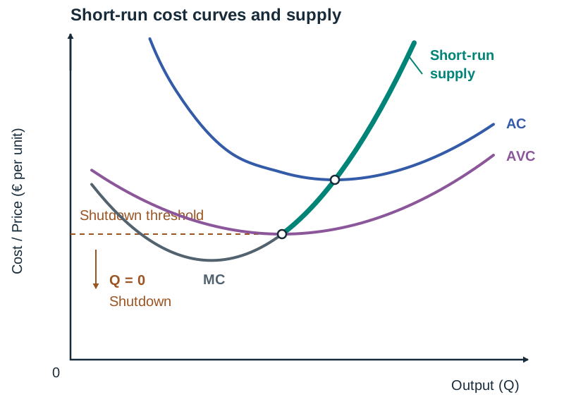
This explains why supply curves slope upwards: because diminishing marginal returns set in, marginal cost rises as output expands. A higher market price is necessary to make producing those extra, more costly units profitable.
Revenue Concepts for Price Takers and Price Makers
Revenue is the money a firm receives from selling its output, before any costs are deducted:
- Total Revenue (TR): All the money received from sales: TR = P × Q.
- Average Revenue (AR): Revenue per unit sold: AR = TR ÷ Q = (P × Q) ÷ Q = P. Because average revenue always equals selling price, the average revenue curve is the demand curve facing the firm.
- Marginal Revenue (MR): The extra revenue gained by selling one additional unit: MR = change in TR ÷ change in Q.
Price Takers vs Price Makers
- Price Takers (Perfect Competition): The firm is too small to influence the market price and can sell any quantity at the going market rate. Because price is constant regardless of output, Price = AR = MR. The revenue curve is a horizontal line. Total revenue is a straight diagonal line rising steadily from the origin.
- Price Makers (Monopoly, Oligopoly, Monopolistic Competition): To sell a higher quantity, the firm must lower its selling price. When the firm faces a linear downward-sloping demand curve, marginal revenue lies below average revenue and falls twice as steeply.
The gap exists because cutting the price to sell one extra unit also cuts the price on every unit the firm could already have sold at the higher price. So the extra revenue from the last unit (MR) is less than the price it sells for (AR).
Revenue Schedule for a Price Maker
Consider a firm that must lower its price by €1 for every additional unit it seeks to sell:
| Price (€) / AR | Quantity | TR (€) | MR (€) |
|---|---|---|---|
| 10 | 1 | 10 | 10 |
| 9 | 2 | 18 | 8 |
| 8 | 3 | 24 | 6 |
| 7 | 4 | 28 | 4 |
| 6 | 5 | 30 | 2 |
| 5 | 6 | 30 | 0 |
| 4 | 7 | 28 | −2 |
Three key observations earn marks here:
- AR equals price at every output level (AR = TR ÷ Q).
- MR lies below AR for all units after the first and falls twice as fast (dropping by €2 each time while price drops by €1).
- TR increases while MR is positive, reaches its maximum (€30) where MR = 0, and begins to fall once MR turns negative.
Drawing Cost and Revenue Diagrams, Equilibrium, and the Long Run
Profit is the difference between total revenue and total cost: Profit = TR − TC = (AR − AC) × Q.
The Two Conditions for Profit Maximisation
A firm maximises profit at the output where:
- MC = MR.
- MC must be rising at that output (MC cuts MR from below).
The second condition is essential because a tick-shaped MC curve can cross MR twice. At the first intersection MC is falling, meaning producing extra units adds more to revenue than to cost. Stopping there would forfeit profit. The true profit maximum occurs only where MC is rising.
Drawing and Labelling the Diagram
Put Costs and Revenue (€) on the vertical axis and Output (Q) on the horizontal axis. Label both axes clearly.
- MC: Falls at first, hits a minimum, then rises steeply—resembling a tick shape.
- AVC: U-shaped. MC cuts AVC at its lowest point.
- AC: U-shaped and always sits above AVC. The vertical gap between AC and AVC is AFC, meaning the two curves draw closer together as output rises. MC cuts AC at the lowest point of AC, to the right of the AVC minimum.
- Price taker: AR = MR = Price, drawn as a horizontal line.
- Price maker: AR slopes downwards; MR lies below AR, is twice as steep, and hits the horizontal axis halfway to the AR intercept.
Follow these four steps to read the firm's equilibrium position:
- Locate where MC cuts MR from below. Drop a vertical dotted line to the horizontal axis to mark output Q1.
- Extend that vertical line up to the AR curve, then read across to the vertical axis to find price P1.
- From the point where the vertical line cuts the AC curve, read across to the vertical axis to find unit cost C1.
- Shade the rectangle bounded by P1, C1, and Q1.
- If P1 > C1, the shaded rectangle is supernormal profit = (AR − AC) × Q.
- If C1 > P1, the rectangle is an economic loss = (AC − AR) × Q.
- If P1 = C1 (the AR curve just touches the AC curve at Q1), there is no rectangle: the firm earns normal profit only. For a price taker, whose AR line is horizontal, this touching point is the minimum of AC; for a price maker, whose AR slopes downwards, it lies to the left of the AC minimum.
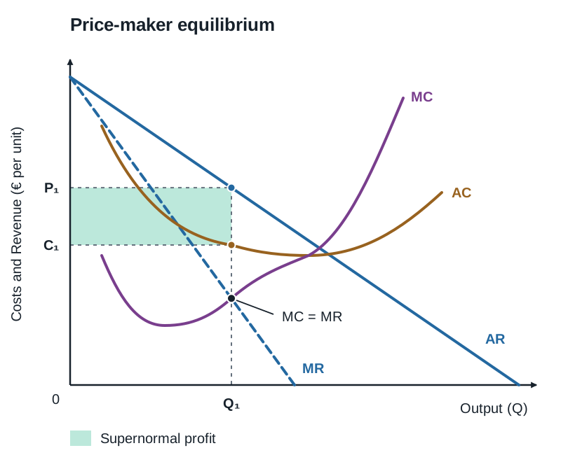
Using totals instead: profit is greatest where the vertical distance between the TR curve and the TC curve is at its widest, provided TR lies above TC.
Short-Run Shutdown vs Long-Run Entry and Exit
In the short run, fixed costs must be paid even if output stops:
- If AR > AVC: The firm covers all its variable costs and each unit sold makes a contribution towards fixed costs, so producing gives a smaller loss than closing.
- If AR = AVC: There is no contribution—the loss equals fixed costs whether the firm produces or not. This is the shutdown point.
- If AR < AVC at every output: Producing makes the loss bigger than fixed costs, so the firm shuts down immediately in the short run.
The long run determines whether the firm remains in the industry:
- Supernormal profit (AR > AC): In markets with low barriers to entry, new firms enter. Market supply increases, market price and the firm's AR curve fall, and entry continues until AR = AC, where only normal profit is earned.
- Loss (AR < AC): If price does not recover, firms exit once fixed contracts (leases, loans) expire. Market supply decreases, market price rises, and exit stops when surviving firms earn normal profit again.
- Blocked entry: Where high entry barriers exist (patents, massive capital requirements), supernormal profit can persist indefinitely in the long run.
The Long Run: Economies, Diseconomies, and Why Small Firms Survive
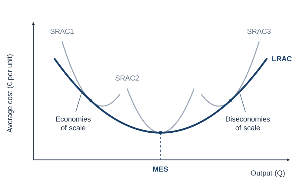
In the long run, all factors of production are variable and the firm can change its overall operational capacity. The Long-Run Average Cost (LRAC) curve acts as an envelope wrapping around all possible short-run average cost curves. The lowest point of a short-run AC curve shows cost minimisation for that single factory size; the minimum point of the LRAC curve represents overall productive efficiency for the firm.
- Internal economies of scale occur when expanding the firm's own output lowers its long-run average cost per unit.
- Internal diseconomies of scale occur when expanding scale beyond optimal capacity causes long-run average cost to rise.
- Minimum Efficient Scale (MES): The lowest output level where a firm achieves minimum long-run average cost.
Short Run vs Long Run Cost Drivers
| Feature | Law of Diminishing Marginal Returns | Economies and Diseconomies of Scale |
|---|---|---|
| Time Horizon | Short run (at least one factor is fixed) | Long run (all factors of production are variable) |
| Core Mechanism | Variable inputs crowd a fixed plant or premises | Altering the firm's overall scale of operations |
| Cost Impact | Causes short-run MC, AVC, and AC curves to rise | Causes LRAC to fall (economies) then rise (diseconomies) |
Examiners often ask you to distinguish the two, and mixing them up loses the explanation marks for the whole part.
Internal Economies of Scale
- Purchasing (Bulk-Buying): Large buyers negotiate volume discounts on raw materials (e.g. Musgrave or Tesco buying groceries).
- Technical: Large plants install automated processing lines that reduce unit operating costs (e.g. Kerry Group or Glanbia dairy plants).
- Financial: Established firms with assets obtain bank loans at lower interest rates or issue shares cheaply.
- Managerial: Growing enterprises employ dedicated specialists for logistics, HR, and marketing, raising operational efficiency.
- Marketing: Large advertising campaigns cost roughly the same whether a company sells 5,000 or 500,000 units, lowering marketing cost per unit.
Internal Diseconomies of Scale
- Communication Breakdowns: Layers of management delay and distort operational messages.
- Bureaucracy and Coordination Bottlenecks: Lengthy sign-off procedures slow decision-making.
- Worker Alienation: Staff in massive corporations feel disconnected from leadership, leading to lower morale, absenteeism, and lower productivity.
External Economies and Diseconomies of Scale
External economies of scale lower long-run average costs for all firms in an industry due to the growth of the industry in a specific region:
- Specialised labour pool: The pharma cluster in Ringaskiddy, Cork, encourages UCC and MTU to run specialised biotechnology courses, cutting hiring and training costs for all local firms.
- Ancillary services: Specialist maintenance and calibration contractors locate nearby, shortening component lead times.
External diseconomies of scale occur when an industry grows too concentrated in one area, driving up costs for every business in that location:
- Rising input prices: Data centres and tech companies clustering in West Dublin compete for the same specialised engineers and commercial plots, pushing up local wages, rents, and site costs.
- Congestion: Traffic gridlock around industrial parks lengthens transport delivery schedules and raises fuel costs per delivery.
- Pressure on infrastructure: Competition for electricity grid capacity, water connections, and local housing inflates operational expenses.
Why Many Irish Firms Remain Small
Large corporations do not take over every market. Many Irish firms stay small because:
- Size of the market: Demand is local or limited (a rural filling station, a local physiotherapy practice), leaving no volume to spread large fixed overheads across.
- Personal service is the product: In hairdressing, dentistry, and accounting, clients pay for individual attention and personal trust, which cannot be mass-produced.
- Lack of finance: Small businesses lack collateral and cannot issue public shares, so expansion is restricted to retained earnings.
- Owner's preference: Many entrepreneurs choose to retain full independence, avoid debt, and maintain work-life balance rather than chase growth.
- Scale economies exhausted early: In activities where a modest workshop and a van achieve minimum unit costs (low MES), further expansion creates managerial headaches rather than cost savings.
- Niche demand: Customers pay high prices for craftsmanship and local provenance (West Cork artisan cheese, microbreweries), which would be compromised by mass factory production.
Critique of Objectives Beyond Profit Maximisation
Economists assume firms maximise profit because it gives a clear, testable prediction about output. In practice, the managers who run firms often pursue other goals:
- Sales Revenue Maximisation: Management aims to maximise total cash turnover by producing where MR = 0. This results in higher output and a lower price than profit maximisation. Directors often favour sales revenue because executive compensation, bonuses, and prestige are linked to company turnover rather than net profit margins.
- Growth and Market Share Dominance: Firms may deliberately cut prices and accept AR below AC in the short run to squeeze out competitors and capture market share. Ryanair followed this strategy for decades, offering rock-bottom fares to build passenger volume, secure airport fee discounts, and dominate European routes.
- Short-Run Survival: During economic downturns or start-up phases, management's primary focus shifts to covering variable costs (producing where AR ≥ AVC) to maintain cash flow and avoid insolvency, putting profit goals aside.
- Satisficing and the Principal-Agent Problem: In public limited companies, ownership (shareholders seeking maximum dividends) is separated from operational control (salaried managers). This division often leads to 'satisficing'—managers target an acceptable profit level that keeps shareholders satisfied while avoiding excess workload, protecting job security, and preserving managerial perks.
- Corporate Social Responsibility (CSR) and Sustainability: Commercial firms increasingly accept higher input costs to meet ethical and environmental benchmarks. Examples include food processors committing to certified sustainable farming standards, or retailers paying a living wage and eliminating single-use plastics to protect brand reputation.
Evaluation
Many alternative objectives can be interpreted as long-run profit maximisation. Sacrificing short-term margin to secure market dominance or protect environmental credentials builds a loyal customer base that delivers stronger profits in the future. Furthermore, real-world firms rarely possess the perfect data required to pinpoint exact marginal costs and revenues, making profit maximisation a useful general guide to how firms behave rather than a calculation managers actually carry out every day.
Key terms
- Fixed Costs (FC)
- Production costs that do not change as output changes in the short run and must be paid even if output is zero.
- Variable Costs (VC)
- Production costs that alter directly in response to changes in the quantity of output produced.
- Marginal Cost (MC)
- The addition to total cost resulting from producing one extra unit of output: MC = change in TC ÷ change in Q.
- Average Total Cost (ATC / AC)
- Total production cost divided by the quantity produced: AC = TC ÷ Q = AFC + AVC.
- Average Variable Cost (AVC)
- Total variable cost divided by the quantity produced: AVC = VC ÷ Q.
- Total Revenue (TR)
- The total money received from sales: TR = Price × Quantity.
- Average Revenue (AR)
- Total revenue divided by quantity sold (AR = TR ÷ Q = Price); the AR curve represents the demand curve facing the firm.
- Marginal Revenue (MR)
- The addition to total revenue generated by selling one extra unit of output: MR = change in TR ÷ change in Q.
- Law of Diminishing Marginal Returns
- The short-run principle that adding successive units of a variable factor to a fixed factor eventually causes the extra output per additional unit of the variable input to decline.
- Normal Profit
- The minimum return needed to keep the entrepreneur in their current line of business in the long run; included in the AC curve as an implicit economic cost.
- Supernormal Profit
- Any profit earned in excess of normal profit, occurring when Average Revenue exceeds Average Cost (AR > AC).
- Shutdown Point
- The operating position where AR = AVC; if price falls below this point, the firm closes immediately in the short run to cap losses at fixed costs.
- Internal Economies of Scale
- Reductions in long-run average cost achieved by an individual firm through expanding its own scale of operations.
- External Economies of Scale
- Reductions in long-run average cost enjoyed by all firms in an industry due to the growth and concentration of that industry in a geographic hub.
- External Diseconomies of Scale
- Increases in long-run average cost experienced by all firms in an industry when the industry becomes overly concentrated in one geographic area.
- Minimum Efficient Scale (MES)
- The lowest level of output at which a firm reaches minimum long-run average cost.
- Satisficing
- A corporate behaviour where salaried managers aim for an acceptable target profit to keep shareholders content rather than striving for the absolute maximum.
- Price Taker
- A firm operating in a perfectly competitive market that has no power over market price and faces a horizontal demand line where Price = AR = MR.
- Price Maker
- A firm that exercises pricing power and faces a downward-sloping demand curve, where selling more requires lowering the price, causing MR to lie below AR.
Check yourself
A firm has a Total Cost of €800 at zero output and €3,200 when producing 400 units. What are its Total Fixed Cost, Total Variable Cost, and Average Variable Cost at 400 units?
Total Fixed Cost is €800 (TC at Q = 0). Total Variable Cost = €3,200 − €800 = €2,400. Average Variable Cost = €2,400 ÷ 400 = €6.00 per unit.
A firm sells 3 units at €8 each and 4 units at €7 each. Calculate Marginal Revenue for the fourth unit.
TR at 3 units = €8 × 3 = €24. TR at 4 units = €7 × 4 = €28. Marginal Revenue = €28 − €24 = €4. Note that MR (€4) is lower than the selling price (€7).
If Marginal Cost is currently €24 and Average Total Cost is €19, what will happen to Average Total Cost if the firm produces one more unit?
Average Total Cost will rise, because the marginal unit costs more (€24) than the running average (€19), pulling the average upward.
What are the two conditions required for a firm to maximise profit?
1. Marginal Cost must equal Marginal Revenue (MC = MR). 2. Marginal Cost must be rising at that output, meaning the MC curve cuts the MR curve from below.
A firm sells 250 units at €40 each. Its Average Variable Cost is €30 and its Average Total Cost is €48. Should this firm produce in the short run? Justify your answer.
Yes, it should continue producing. Although it incurs a loss of €8 per unit (AR €40 < ATC €48), price (€40) exceeds AVC (€30). Each unit makes a €10 contribution towards fixed overheads, making the operating loss smaller than shutting down.
What is an external diseconomy of scale? Give one Irish example.
An external diseconomy of scale occurs when the long-run average costs of all firms in an industry increase because the industry has become overly concentrated in one geographic area. Example: Tech firms and data centres clustering in West Dublin competing for the same specialist staff and land, pushing up wages, commercial rents, and site costs for all businesses in that hub.
Why does a competitive market earn only normal profit in the long run?
Because of free entry and exit. If firms earn supernormal profit, new entrants join the market, increasing supply and reducing market price until AR = AC. If firms make losses, businesses exit once fixed commitments expire, reducing supply and raising price back to AR = AC.