Optimal & Critical Paths

Networks, Terminology, and What 'Optimal' Means

A network (or graph) is a collection of vertices (or nodes) joined by edges (or arcs). In an undirected network, edges can be traversed in both directions. In a directed network, edges are arrows indicating one-way movement. A path is an unbroken sequence of edges connecting a sequence of vertices without repeating any vertex.

A cycle is a closed path that starts and finishes at the same vertex without repeating any edge. A network containing no cycles is described as acyclic. A graph is connected if there is at least one path between every pair of vertices. If some vertices cannot be reached from the rest, the network is disconnected. Dijkstra's algorithm only computes distances to nodes within the same connected component as the source.

Every edge carries a numerical weight, representing a physical metric such as distance, travel time, financial cost, or capacity. Depending on the scenario, optimal has different meanings:

• In routing problems, optimal typically means finding a shortest path to minimise total travel time, distance, or cost.
• In project scheduling, optimal refers to determining the minimum project completion time by identifying the critical path, which is the longest-duration path of dependent tasks through the network.

Comparing Shortest-Route Techniques

The Leaving Certificate syllabus requires evaluating different techniques for finding shortest routes:

• Exhaustive search (listing every path): Guarantees finding the global optimum for small networks, but the number of potential paths grows exponentially as nodes increase, making it impractical for large networks.
• Dijkstra's algorithm: Very efficient and determines the shortest route from the source to every node in a single sweep. It requires all edge weights to be non-negative ($w \ge 0$).
• Bellman's dynamic programming: Ideal for problems structured into sequential stages (such as inventory periods or project years). It handles non-edge costs and negative values, and provides the optimal continuation from every intermediate state.

Dijkstra's Shortest Path Algorithm

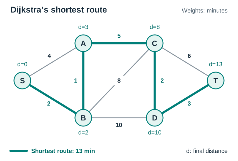
Dijkstra's algorithm is a greedy algorithm that determines the shortest path from a single source vertex to all other vertices in a weighted network where all edge weights are non-negative ($w \ge 0$). If negative weights are present, Dijkstra's algorithm can fail because a subsequent negative edge could make an already settled path shorter.

Recording Your Work Clearly

Most marks in a Dijkstra question are awarded for your working method. You must keep track of three values at every node:

1. Order of labelling: The sequence number in which the vertex is permanently settled (beginning with 1 at the source).
2. Final value: The confirmed shortest cumulative distance from the source.
3. Working values: Provisional distances calculated from adjacent permanently labelled nodes. When a smaller working value is found, cross out the old value neatly and record the new one beside it, noting the predecessor node.

A clear way to show this at each node is a three-part layout:

+-----------------------+---------------------+
|  Order of labelling   |     Final value     |
+-----------------------+---------------------+
|  Working values: 10(B), 8(A)                |
+---------------------------------------------+

Step-by-Step Procedure

1. Set the source node to Order 1 with a permanent final value of 0.
2. From the node $u$ just made permanent, calculate candidate distances to every unlabelled neighbouring node $v$ directly connected to it:

In a directed network, only follow edges pointing in the direction of the arrow. If the candidate value is strictly less than $v$'s existing working value (or if $v$ has none yet), update $v$'s working value to this candidate.

1. Inspect all unlabelled vertices across the entire network. Select the vertex with the smallest working value and declare it permanent. Assign it the next sequential order number and record that working value as its final value. If there is a tie for the smallest value, either node may be chosen next.
2. Repeat steps 2 and 3 until the destination vertex is made permanent.
3. Trace backwards from the destination to find the path. An edge from $u$ to $v$ lies on a shortest path if:

If more than one predecessor satisfies this equation, multiple shortest paths of identical length exist.

Dynamic Programming and Bellman's Principle

Dynamic programming solves complex multi-stage decision problems by decomposing them into smaller subproblems. It relies on Bellman's Principle of Optimality:

An optimal policy has the property that whatever the initial state and initial decision are, the remaining decisions must constitute an optimal policy with regard to the state resulting from the first decision.

In plain English, every section of an optimal path must itself be optimal. If the cheapest route from Dublin to Galway passes through Athlone, the Athlone-to-Galway portion must be the cheapest possible way to travel between those two points. If a cheaper path from Athlone to Galway existed, substituting it would reduce the overall journey cost, contradicting the claim that the initial route was optimal.

Algebraic Formulation

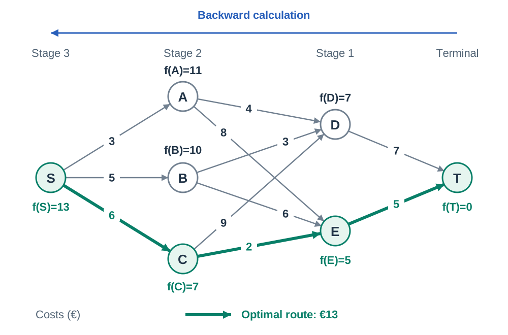
Dynamic programming operates by backward induction — working from the terminal destination backwards to the source across a weighted directed acyclic network. Let $f(x)$ denote the optimal (minimum) cost from state $x$ to the destination $T$:

Where $w(x, y)$ is the immediate cost of transitioning from state $x$ to state $y$, and $f(y)$ is the optimal cost from state $y$ onwards. For maximisation problems, replace $\min$ with $\max$.

Setting Out the Table

Define your stage, state, and action in words before calculating. A standard layout uses five columns:

• Stage ($n$): The decision step, conventionally indexed by the number of stages or time periods remaining until the horizon.
• State ($s$): The physical condition, location, or available stock at the start of the stage.
• Action ($x$): The decision taken.
• Destination ($s'$): The resulting state in the next stage.
• Value: The combined payoff: $\text{Immediate Cost/Profit} + f(s')$.

Mark the optimal choice for each state with an asterisk ($*$). When the table is complete, trace the optimal policy forward from the initial state.

Dynamic Programming Archetypes

The Leaving Certificate specification identifies four distinct applications of dynamic programming:

1. Multi-Stage Routing

Finding the cheapest or quickest route through a directed acyclic network. Stages represent steps remaining, states represent junctions, and actions represent the chosen edge. The value is calculated as $\text{Immediate Cost} + f(\text{destination})$.

2. Stock Control (Inventory Management)

Determining monthly production to meet known customer demand while minimising the sum of production setups, unit costs, and storage fees.

• State ($s$): Opening stock at the start of the month.
• Action ($x$): Number of units manufactured.
• Destination ($s'$): Closing stock carried into the next month, governed by:

• Value: $\text{Setup Cost} + \text{Unit Cost} + \text{Storage}(s') + f(s')$.

3. Allocation of Resources

Distributing a fixed, finite resource (such as capital or raw materials) across competing divisions to maximise total profit.

• Stage: Product line or project being funded.
• State ($s$): Units of resource still available to allocate.
• Action ($x$): Units allocated to the current product ($0 \le x \le s$).
• Destination ($s'$): Units remaining for subsequent stages ($s' = s - x$).
• Value: $\text{Profit}(x) + f(s - x)$.

For example, if 4 tonnes of raw material remain for two divisions, allocating 1 tonne to division A gives a profit of €120. If the optimal profit from allocating the remaining 3 tonnes to division B is $f(3) = €250$, the value is $120 + 250 = €370$.

4. Equipment Replacement and Maintenance

Deciding when to replace an asset over an $N$-year horizon to minimise overall net expenditure.

• Asset bought new each cycle: If a new asset is purchased and kept for $k$ years before trade-in, compute the cycle cost $c(k)$ first:

The recurrence relation with $n$ years remaining is $f(0) = 0$ and $f(n) = \min_{k} \{ c(k) + f(n - k) \}$.

• Asset already owned: If the firm currently owns an asset, let the state be the age of the asset at the start of the year, and stage be years remaining. The two actions are Keep (pay that year's maintenance; age increases by 1) or Replace (trade in at resale value, pay new purchase price, pay year-1 maintenance; age becomes 1 next stage).

Project Scheduling: Networks and Passes

A project consists of interdependent activities. We model this using an activity-on-arc network, where directed arrows represent activities (with durations) and event nodes represent milestone moments in time.

Examination Question Structure

A 50-mark project scheduling question typically follows a set sequence of tasks:

1. Draw the network from the precedence table using dummy activities where necessary.
2. Carry out the forward pass to determine early times.
3. Carry out the backward pass to determine late times.
4. Complete the float table for all activities.
5. State the critical path(s) and minimum project completion time.
6. Interpret the effect of delays or scheduling changes on the project completion date.

Drawing from Precedence Tables and Dummies

• Ensure the network has exactly one source node (start) and one sink node (finish).
• Number event nodes so that every directed arc goes from a lower-numbered node to a higher-numbered node.
• A dummy activity (duration 0, drawn as a dashed line) is needed in two situations:

1. Logical dependency: Activity C depends on A and B, but activity D depends only on A. Drawing a dummy from the end of A to the start of C enforces this without delaying D.
2. Uniqueness: Two activities share the same start and finish events. Because an activity must be uniquely identified by its pair of events $(i, j)$, a dummy separates their terminal nodes.

Calculating Event Times

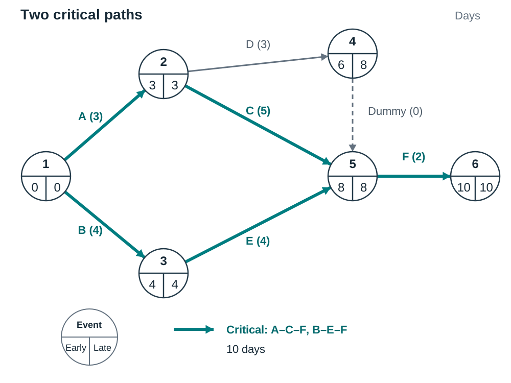
Every event circle is split into the early time (or earliest event time, EET) and the late time (or latest event time, LET).

• Forward Pass (Early Times): Set $\text{early time}_{\text{source}} = 0$. Moving forward from source to sink:

Take the maximum where paths converge, because an event cannot occur until the slowest prerequisite activity finishes. The early time of the sink gives the minimum project completion time.

• Backward Pass (Late Times): Set $\text{late time}_{\text{sink}} = \text{early time}_{\text{sink}}$. Moving backward from sink to source:

Take the minimum where paths diverge backwards, because each event must occur early enough to meet the tightest subsequent deadline. Always check that $\text{late time}_{\text{source}} = 0$.

Total Float, Critical Paths, and Delays

For an activity running from event $i$ to event $j$ with duration $t$:

• Earliest start: $\text{early time}_i$
• Earliest finish: $\text{early time}_i + t$
• Latest finish: $\text{late time}_j$
• Latest start: $\text{late time}_j - t$

Total Float

The total float is the maximum duration an activity can be delayed without delaying the entire project:

Critical Paths

An activity is a critical activity if and only if its total float is 0:

High-Level Distinction: Having $\text{early time} = \text{late time}$ at both end nodes is a necessary condition, but not a sufficient condition. For instance, if event 1 has early and late times of 0, event 4 has early and late times of 10, and an activity connecting them takes 7 days, its float is $10 - 0 - 7 = 3$ days. The activity is not critical despite running between two critical events.

The critical path is a continuous sequence of zero-float activities from the source node to the sink node. It is the longest-duration path through the network and dictates the minimum project completion time.

Evaluating the Effect of Delays

If an activity with total float $F$ is delayed by $d$ time units:

• If $d \le F$, the overall project duration is unchanged, although other activities sharing that float window may lose flexibility.
• If $d > F$, the project completion time increases by $d - F$ time units, and the critical path may shift to run through that delayed activity.

Gantt Charts

A Gantt chart plots activities on a horizontal time axis. Each activity is drawn as a solid bar starting at its earliest start time for its duration, followed by a dashed line showing its total float up to its latest finish. A vertical line at time $t$ shows which activities must be happening (critical activities) and which could be happening (non-critical activities whose float window spans $t$).

Key terms

Dijkstra's Algorithm

A greedy algorithm that finds the shortest path from a single source vertex to all other vertices in a network with non-negative edge weights by iteratively giving permanent labels to nodes with the smallest working values.

Bellman's Principle of Optimality

The principle that an optimal policy has the property that, whatever the initial state and decision are, the remaining decisions must constitute an optimal policy with regard to the state resulting from the first decision.

Stage

A distinct step or time period in dynamic programming, numbered in reverse order by the number of decisions or time units remaining.

State

The physical condition, location, asset age, or inventory level of the system at the start of a dynamic programming stage.

Action

A feasible decision chosen from a state that transitions the system into a destination state at the subsequent stage.

Optimal Policy

The complete sequence of optimal decisions specifying the best action to take from every state across all stages to achieve the global optimum.

Early Time

The earliest possible time an event milestone can occur (also called earliest event time, EET), determined on the forward pass by taking the maximum of incoming (early time + duration).

Late Time

The latest possible time an event milestone can occur without extending the project duration (also called latest event time, LET), found on the backward pass by taking the minimum of outgoing (late time - duration).

Total Float

The amount of time an activity can be delayed without delaying the completion of the overall project, given by late time of finish event - early time of start event - duration.

Critical Path

A continuous sequence of zero-float activities from the source event to the sink event that determines the minimum project completion time; it is the longest-duration path through the project network.

Dummy Activity

A zero-duration, zero-cost directed dashed arc used in an activity-on-arc network to preserve unique node numbering or enforce logical dependencies without adding unnecessary constraints.

Cycle

A closed path in a network that starts and finishes at the same vertex without repeating any edge. A network without cycles is acyclic.