Further Integration (u-substitution, integration by parts)

Kinematics, Acceleration Forms, and Deriving Constant-Acceleration Formulae

When analyzing particle motion, acceleration can be expressed in two calculus forms depending on the variables you need to connect:

• When relating velocity and time ($v, t$), use a = dv/dt.
• When relating velocity and displacement ($v, s$), apply the chain rule: $a = \frac{dv}{dt} = \frac{dv}{ds}\frac{ds}{dt} = v\frac{dv}{ds}$, giving a = v dv/ds.

Deriving the Kinematic Formulae Using Calculus

Strand 3 explicitly requires deriving the standard constant-acceleration equations from first principles using calculus. Take acceleration $a$ as constant, with initial conditions $v = u$ and $s = 0$ at $t = 0$.

1. Velocity after time t ($v = u + at$): Start from $a = \frac{dv}{dt}$. Separate the variables and integrate:

At $t = 0$, $v = u$, so $c = u$. This gives:

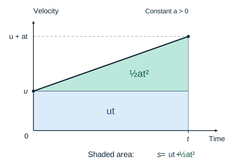
2. Displacement after time t ($s = ut + \frac{1}{2}at^2$): Since $v = \frac{ds}{dt} = u + at$, separate variables:

At $t = 0$, $s = 0$, so $c = 0$. This gives:

3. Velocity after displacement s ($v^2 = u^2 + 2as$): When time is absent, write $a = v\frac{dv}{ds}$. Separate variables and integrate:

At $s = 0$, $v = u$, so $c = \frac{1}{2}u^2$. Multiplying through by 2 gives:

Displacement Versus Distance Travelled

Integrating velocity over a time interval gives displacement: $s = \int_{t_1}^{t_2} v(t)\,dt$. If the velocity changes sign during the motion, the particle reverses direction and forward and backward displacements cancel out. To calculate the total distance travelled, find the turning times where $v(t) = 0$, integrate over each interval separately, and add their absolute values:

Integration by Substitution and Resisted Motion

Integration by substitution turns a composite integral into a standard form found in the Formulae and Tables booklet. It reverses the chain rule of differential calculus.

Theoretical Derivation

Let $F(u)$ be an antiderivative of $f(u)$ such that $F'(u) = f(u)$, and let $u = g(x)$. By the chain rule:

Integrating both sides with respect to $x$ gives:

Four Steps for Substitution

1. Select an inner function $u = g(x)$ whose derivative appears elsewhere in the integrand as a multiplying factor.
2. Differentiate to get $du = g'(x)\,dx$, so $dx = \frac{du}{g'(x)}$.
3. Substitute completely so no trace of $x$ remains. If an extra power of $x$ remains, rearrange $u = g(x)$ to express $x$ in terms of $u$.
4. For indefinite integrals, integrate and back-substitute $u$. For definite integrals, convert the limits immediately: $u_1 = g(a)$ and $u_2 = g(b)$, then evaluate directly in terms of $u$.

Two Ways to Handle Constants of Integration

When solving dynamical differential equations via separation of variables, you can either:

• Integrate indefinitely and solve for the constant $+ c$ using initial conditions, or
• Set up definite integrals directly between physical limits (for example, $\int_u^v \dots dv = -\int_0^s \dots ds$). The definite-integral route avoids losing constants, but if you substitute $w = g(v)$ on the left, you must convert the velocity limits into $w$-limits before evaluating.

Resisted Motion with Respect to Time and Terminal Velocity

A particle of mass $m$ falling from rest under gravity subject to linear resistance $kv$ satisfies:

Separate variables:

Letting $u = mg - kv$ gives $du = -k\,dv$, so the left side integrates to $-\frac{1}{k}\ln|mg - kv|$. With $v = 0$ at $t = 0$:

Terminal velocity is the constant speed achieved when the resistive drag balances the driving force, meaning acceleration is zero. Setting $\frac{dv}{dt} = 0$ in the equation of motion gives:

Taking the limit of $v(t)$ as $t \to \infty$ yields $v \to \frac{mg}{k}$, confirming the terminal speed.

Integration by Parts: Selection, Layout, and Repeated Application

Integration by parts is used when the integrand is a product of two distinct function families where one is not the derivative of the other. It reverses the product rule of differentiation.

Theoretical Derivation

The product rule states:

Integrating both sides with respect to $x$:

Rearranging yields the standard formula:

Notation note: In mechanics, write the second variable as $w$ rather than $v$ to avoid confusing it with velocity.

Selecting u via LIATE

Choose $u$ as the function that simplifies most when differentiated, using the priority list LIATE:

• L: Logarithmic functions (e.g. $\ln x$)
• I: Inverse trigonometric functions (e.g. $\tan^{-1}x$)
• A: Algebraic polynomials (e.g. $x, t^2, 3s$)
• T: Trigonometric functions (e.g. $\sin x, \cos 2x$)
• E: Exponential functions (e.g. $e^{kx}, e^{-t}$)

In Applied Mathematics kinematics, the choice is almost always between an algebraic term and an exponential or trigonometric term: the polynomial becomes $u$, and the remaining term including $dt$ becomes $dw$.

Repeated Integration by Parts

If $u$ is an algebraic power $t^n$ with $n > 1$, parts must be applied $n$ times in succession. Keep minus signs inside brackets to avoid sign errors.

Worked example of repeated parts: A particle has velocity $v(t) = t^2 e^{-t}\,\text{m s}^{-1}$, with $s(0) = 0$. Find $s(t)$.

• First application: let $u = t^2 \implies du = 2t\,dt$, and $dw = e^{-t}\,dt \implies w = -e^{-t}$.

• Second application on $\int t e^{-t}\,dt$: let $u = t \implies du = dt$, and $dw = e^{-t}\,dt \implies w = -e^{-t}$.

• Combining terms:

Using $s(0) = 0$: $0 = -e^0(0 + 0 + 2) + c \implies c = 2$. Thus, $s(t) = 2 - e^{-t}(t^2 + 2t + 2)\,\text{m}$.

Strategic Recognition: The Look-Alike Decision Table

Many integrals in mechanics look superficially similar but require entirely different techniques. Inspecting the algebraic relationship between the numerator and denominator or between factors determines the correct method.

When an examination question states 'using integration by parts or otherwise', any valid method receives full marks, but the stated technique is virtually always the intended and fastest route.

Work, Energy, and Conservative Forces by Integration

When a force varies with position, work done cannot be evaluated by simple multiplication. It is defined by the definite integral of force along the displacement path:

Deriving the Work–Energy Theorem by Integration

Strand 3 requires explaining how kinetic energy relates to work done. Substitute Newton's second law $F = ma$ into the work integral and write acceleration as $a = v\frac{dv}{ds}$:

This proves the work–energy theorem: the work done by the resultant force equals the change in kinetic energy ($W_{\text{net}} = \Delta E_k$). Note that the change of variable from $ds$ to $dv$ converts position limits into velocity limits, directly illustrating integration by substitution.

For an object falling a height $h$ under gravity alone, $W = \int_0^h mg\,ds = mgh$, which equals the decrease in gravitational potential energy.

Elastic Potential Energy: Springs and Elastic Strings

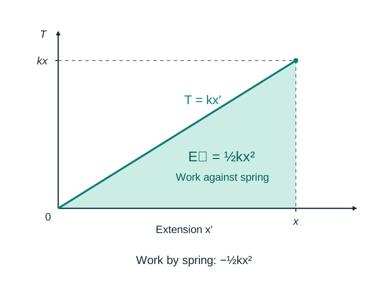
Hooke's Law states that the tension in an elastic spring or string is proportional to its extension $x$ beyond its natural length $l$:

where $k$ is the spring stiffness and $\lambda$ is the elastic modulus. Because tension pulls back towards the natural length, the force exerted on the particle by the spring is $-kx$.

The work done against the elastic restoring force to stretch the spring from extension $0$ to $x$ represents the elastic potential energy stored:

The work done by the spring on the particle during this extension is therefore $-\frac{1}{2}kx^2$.

Key terms

Integration by Substitution

An analytical calculus technique derived by reversing the chain rule, where setting $u = g(x)$ transforms $\int f(g(x))g'(x)\,dx$ into $\int f(u)\,du$.

Integration by Parts

An analytical calculus technique derived by reversing the product rule, evaluated using the identity $\int u\,dw = uw - \int w\,du$.

Separation of Variables

The method of solving a first-order differential equation by rearranging terms so that each variable and its differential appear exclusively on opposite sides before integrating.

Terminal Velocity

The constant maximum speed attained by an object moving through a resisting fluid when the drag force equals the driving force, resulting in zero acceleration.

Work–Energy Theorem

The principle that the work done by the resultant force on a particle equals its change in kinetic energy: $W_{\text{net}} = \int F\,ds = \frac{1}{2}mv_2^2 - \frac{1}{2}mv_1^2$.

Hooke's Law

The physical law stating that the restoring tension in an extended elastic string or spring is directly proportional to its extension: $T = kx = \frac{\lambda x}{l}$.

Kinetic Energy

The mechanical energy possessed by an object due to its motion, derived from calculus as $E_k = \frac{1}{2}mv^2$.

Elastic Potential Energy

The mechanical energy stored in a stretched or compressed elastic body, calculated by integrating work done against restoring tension: $E_p = \frac{1}{2}kx^2 = \frac{\lambda x^2}{2l}$.