Differential Equations

Continuous Change and the Modelling Cycle

A differential equation models systems where change occurs continuously over time or distance. This contrasts directly with discrete difference equations, which update values in separate jumps across time steps (such as annual compound interest or species with single annual breeding seasons).

Under Strand 1, applied mathematicians investigate authentic continuous problems through a four-stage modelling cycle:

1. Formulating problems: Identify the core variables (such as time $t$, velocity $v$, displacement $s$, temperature $T$, or population $P$) and make reasonable simplifying assumptions (such as neglecting air buoyancy or treating ambient temperature as constant).
2. Translating into mathematics: Translate the physical law or verbal rate description into calculus notation. For instance, 'the rate of decay is proportional to the mass remaining' becomes $\frac{dm}{dt} = -km$, where $k > 0$.
3. Computing solutions: Separate variables, integrate using standard calculus techniques, and determine integration constants using initial or boundary conditions.
4. Evaluating and reporting: Check whether the mathematical output makes physical sense. Check that the sign and magnitude are realistic, test limiting behaviour as $t \to \infty$, check sensitivity to parameters, and compare predictions with experimental or historical data.

First-Order Separable Equations and Integration Tools

A first-order differential equation has a first derivative as its highest derivative. An equation is separable if it can be written with the variables split on either side of the equals sign:

Integrating both sides produces a general solution containing an arbitrary constant $+ C$. Given initial conditions (such as $y = y_0$ when $x = x_0$), evaluate $C$ to produce the unique particular solution.

Applying definite integration limits directly to match the initial and final states avoids sign slips and constant-of-integration errors:

Essential Standard Integrals

• $\int \frac{1}{y}\,dy = \ln|y| + C$
• $\int \frac{1}{ay + b}\,dy = \frac{1}{a}\ln|ay + b| + C$
• $\int \frac{y}{a^2 + y^2}\,dy = \frac{1}{2}\ln(a^2 + y^2) + C$
• $\int \frac{1}{a^2 + y^2}\,dy = \frac{1}{a}\tan^{-1}\left(\frac{y}{a}\right) + C$
• $\int \frac{1}{\sqrt{a^2 - y^2}}\,dy = \sin^{-1}\left(\frac{y}{a}\right) + C$
• Partial fractions: $\frac{1}{y(K - y)} = \frac{1}{K}\left(\frac{1}{y} + \frac{1}{K - y}\right)$, which integrates to $\frac{1}{K}(\ln|y| - \ln|K - y|) + C = \frac{1}{K}\ln\left|\frac{y}{K - y}\right| + C$.

Verifying a Solution

When an exam question asks you to show that a given function satisfies a differential equation, do not attempt to solve the equation from scratch. Differentiate the given function the required number of times and substitute directly into the differential equation.

For example, to show that $x = A\sin(\omega t + \varepsilon)$ satisfies $\frac{d^2x}{dt^2} = -\omega^2 x$:

Strand 4 Continuous Rate Models

Many real-world phenomena follow the conservation principle: rate of change = rate in − rate out.

Exponential Growth, Decay, and Finance

• Radioactive decay: $\frac{dN}{dt} = -kN$ integrates to $N(t) = N_0 e^{-kt}$. The half-life is $t_{1/2} = \frac{\ln 2}{k}$.
• Continuous compounding: If an account balance $B$ earns nominal interest rate $r$ compounded continuously, $\frac{dB}{dt} = rB$, so $B(t) = B_0 e^{rt}$ with doubling time $t_d = \frac{\ln 2}{r}$.

Newton's Law of Cooling

Newton's law of cooling states that the rate of change of temperature is proportional to the difference between the body's temperature $T$ and the surrounding ambient temperature $T_s$:

Separating variables gives $\ln|T - T_s| = -kt + C$, which simplifies to $T(t) = T_s + (T_0 - T_s)e^{-kt}$. As $t \to \infty$, $e^{-kt} \to 0$, so $T \to T_s$.

Restricted (Logistic) Growth and Spread of Disease

Unrestricted growth $\frac{dP}{dt} = rP$ predicts infinite population. In reality, food and space impose a carrying capacity $K$:

When $P$ is small, the bracket is close to $1$ (rapid near-exponential growth). As $P \to K$, the growth rate drops to zero. Separating variables requires partial fractions:

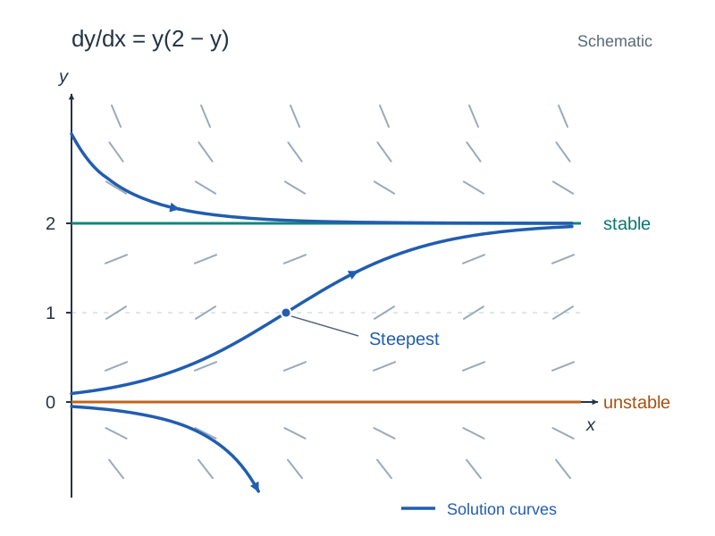
Setting $\frac{dP}{dt} = 0$ gives two equilibria: $P = 0$ (an unstable equilibrium) and $P = K$ (a stable equilibrium).

In an epidemic among a closed population of $N$ individuals, if $I$ are infected and $N - I$ are susceptible, transmission depends on interactions between both groups: $\frac{dI}{dt} = kI(N - I)$. This is identical to the logistic model with carrying capacity $N$. The infection spreads fastest when $I = \frac{N}{2}$, because the product $I(N - I)$ reaches its maximum there.

Harvesting Models

When a population growing at rate $kP$ suffers constant harvesting $H$ (such as logging or fishing), $\frac{dP}{dt} = kP - H = k\left(P - \frac{H}{k}\right)$. The value $P^* = \frac{H}{k}$ is an unstable equilibrium. If $P_0 > \frac{H}{k}$, the stock expands indefinitely. If $P_0 < \frac{H}{k}$, harvesting outstrips reproduction and the population collapses to zero in finite time.

Variable Forces and Kinematics (Strand 3)

When force varies with speed, position, or time, acceleration is not constant. You cannot use the constant-acceleration formulae ($v = u + at$, $s = ut + \frac{1}{2}at^2$, $v^2 = u^2 + 2as$). Instead, use Newton's Second Law: $\sum F = ma$.

Choosing the Expression for Acceleration

• If the question connects velocity and time ($v$ and $t$): use $a = \frac{dv}{dt}$.
• If the question connects velocity and displacement ($v$ and $s$): use the chain rule form $a = v\frac{dv}{ds}$.

Checklist for 'Show That' Mechanics Questions

1. Draw a clear diagram, showing all forces and marking the chosen positive direction.
2. Look at the printed target: if displacement $s$ appears, use $a = v\frac{dv}{ds}$; if time $t$ appears, use $a = \frac{dv}{dt}$.
3. Write $\sum F = ma$, giving every force its correct algebraic sign.
4. Divide across by $m$. When resistance is given as $kmv$, the mass $m$ cancels immediately.
5. Substitute numerical values such as $g = 9.8$ only when the target equation contains specific numbers (such as $29.4$ or $392$).
6. Rearrange algebraically until your equation matches the required examination line.

Terminal Velocity and Fluid Forces

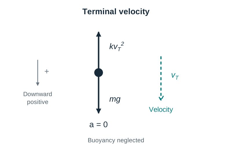
An object moving through a fluid experiences its downward weight $mg$, an upward buoyancy force (upthrust) if submerged, and a resistive drag force opposing motion. For an object falling vertically downwards under quadratic drag $kv^2$:

Terminal velocity occurs when the forces balance so acceleration becomes zero: $mg - kv^2 = 0 \implies v_T = \sqrt{\frac{mg}{k}}$. With linear drag $kv$, setting $mg - kv = 0$ gives $v_T = \frac{mg}{k}$. Always find terminal velocity by setting acceleration to zero in your equation of motion rather than quoting a memorised formula.

Second-Order Equations Reducible to First Order (Higher Level)

At Higher Level, equations involving second derivatives can be solved when they reduce to first order by substitution.

Case 1: Displacement Missing

When an equation contains only $\frac{d^2s}{dt^2}$, $\frac{ds}{dt}$, and $t$, let $v = \frac{ds}{dt}$ and $\frac{dv}{dt} = \frac{d^2s}{dt^2}$. Solve the resulting first-order equation for $v(t)$, then integrate $v = \frac{ds}{dt}$ with respect to $t$ to find displacement $s(t)$.

Case 2: Time Missing (Force Depending on Position)

When acceleration is given as a function of position $x$, substitute $a = v\frac{dv}{dx}$:

For a particle in Simple Harmonic Motion with $\frac{d^2x}{dt^2} = -\omega^2 x$ released from rest at $x = A$:

To find displacement $x$ as a function of time, replace $v$ by $\frac{dx}{dt}$. Since the particle moves inward from $x = A$, choose the negative root:

At $t = 0$, $x = A$, giving $\sin^{-1}(1) = C \implies C = \frac{\pi}{2}$. Therefore $\frac{x}{A} = \sin\left(\frac{\pi}{2} - \omega t\right) = \cos(\omega t)$, leading to the classic result $x = A\cos(\omega t)$.

Qualitative Analysis and Numerical Methods

When an exact algebraic solution cannot be found easily, qualitative and numerical methods describe how the system behaves.

Direction Fields and Stability

A direction field plots small line segments with slope $\frac{dy}{dx} = f(x, y)$ on a coordinate grid. Solution curves follow these slope segments tangentially.

For example, examine $\frac{dy}{dx} = y(2 - y)$:

• Along $y = 0$ and $y = 2$, the slope is $0$. These horizontal lines represent the equilibrium solutions.
• At $y = 1$, the slope reaches its maximum positive value, $1(2 - 1) = 1$.
• For any starting value $0 < y < 2$, the slope is positive, so solutions increase steepest at $y = 1$ before flattening out smoothly as they approach $y = 2$.

An equilibrium is stable if curves approach it from both sides, and unstable if curves diverge away from it.

Euler's Method

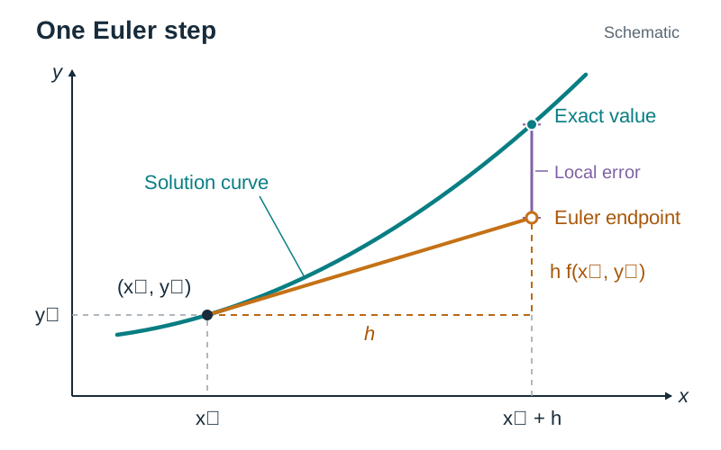
Euler's method follows the solution curve in small steps of fixed width $h$. At each point you work out the slope from the differential equation and move along that straight tangent line to the next point:

This simple recurrence relation is readily implemented in digital tools and spreadsheets. Halving the step size $h$ roughly halves the truncation error. Because tangent lines sit below curves that are concave upward ($\frac{d^2y}{dx^2} > 0$), Euler's method systematically underestimates solutions on curves that bend upwards.

Key terms

Differential Equation

An equation containing an unknown function and one or more of its derivatives, used to model continuous change.

Order

The order of the highest derivative appearing in the equation. For example, dv/dt = -(g + kv) is first order; d²x/dt² = -ω²x is second order.

Separation of Variables

The algebraic technique of rearranging a first-order differential equation so that all terms containing one variable are on one side of the equals sign and all terms containing the other variable are on the opposite side.

General Solution

A solution to a differential equation that includes all possible arbitrary constants of integration, representing an infinite family of curves.

Particular Solution

A specific solution obtained from the general solution by using given initial or boundary values to determine exact numerical values for the arbitrary constants.

Terminal Velocity

The steady maximum speed reached by an object in a fluid when resistive drag and buoyancy forces balance the driving force, resulting in zero acceleration.

Equilibrium Solution

A constant value of the dependent variable where its derivative equals zero, meaning the system experiences no rate of change.

Stable Equilibrium

An equilibrium state where small disturbances decay over time, causing neighbouring solution curves to converge back towards the equilibrium.

Unstable Equilibrium

An equilibrium state where small disturbances grow over time, causing neighbouring solution curves to diverge away from the equilibrium.

Carrying Capacity

The maximum sustainable population that a given environment can support, denoted by K in the logistic growth model.

Half-Life

The time required for a decaying quantity to reduce to exactly half its initial value, calculated as t½ = (ln 2)/k.

Euler's Method

A numerical stepping method that approximates the solution curve of a differential equation along successive tangent lines using yn+1 = yn + h · f(xn, yn).

Relating displacement, velocity and acceleration

The calculus connections linking position s, speed v, and acceleration a, selecting a = dv/dt when working with time and a = v(dv/ds) when working with displacement.