

A difference equation is a rule that tells you how to get the next value in a sequence from the value or values before it — for example, 'next year's population is 1.02 times this year's, minus 150'. Because the rule only applies at whole-numbered steps, difference equations suit anything that is counted or updated at fixed intervals: yearly breeding seasons, monthly repayments, daily case numbers. In this topic you will learn to write such a rule from a description in words, to find a formula for u_n directly in terms of n, to work out terms numerically when no such formula exists, and to say what the answer means for the situation being modelled.
Discrete Change, Sequences, and Differences
Many things in biology, finance, and economics only change at set times — once a year, once a month, or once a day. We number the steps and write for the value at step , so is the starting value, is the value after one step, and so on.
Why a Difference Equation?
When an exam question asks why a difference equation is appropriate rather than a differential equation, state two facts:
- The quantity is recorded and updated at separate, fixed times (such as annually, monthly, or per generation), so the model produces one distinct value for each whole-numbered step.
- A differential equation would be used instead if the quantity changed continuously and smoothly at every instant, such as a cooling liquid or motion under a variable force.
Sequence Differences
The first difference measures the change between consecutive terms:
Taking the difference of consecutive first differences gives the second difference:
Looking at differences lets us identify the underlying formula of a data table:
- Constant first differences (): linear sequence, .
- Constant second differences (): quadratic sequence, .
- Constant third differences: cubic sequence ().
- Constant ratio (): geometric sequence, .
For example, consider the sequence 2, 7, 18, 41, 82:
- First differences: , , ,
- Second differences: , ,
- Third differences: ,
Because the third differences are constant (), the sequence is cubic. We can work forward: the next second difference is , the next first difference is , so the next term is .
Classification and Model Setup
Before solving an equation, you must classify it. In exams, classification marks depend on giving clear reasons rather than just stating labels.
- Order: The difference between the highest and lowest subscripts of the sequence variable. For example, is first order (subscripts differ by 1), whereas is second order (subscripts differ by 2).
- Linearity: An equation is linear if every sequence term () appears only to the first power, terms are not multiplied together, and no sequence term is inside a function like a square root or sine. For example, is linear because depends only on the step number , not on . If an equation contains or , it is non-linear.
- Homogeneity: Collect all terms containing the sequence variable on the left-hand side. If the right-hand side is zero, the equation is homogeneous because there is no term independent of . If an isolated constant, an exponential term, or a polynomial in remains on the right, the equation is inhomogeneous.
Setting Up Timelines and Incremental Models
Always define your timeline before writing an equation: 'Let be the population at the start of year , with at the start of 2024, so .'
Follow the chronological order of events described in the problem:
- If interest is added first and then a payment is deducted: .
- If the payment is deducted at the start of the period before interest is applied: .
A common Leaving Certificate formulation involves successive changes: 'the increase on any day is twice the increase on the previous day'. Translate this directly using first differences:
Rearranging into standard form gives , which is a second-order linear homogeneous equation.
First-Order Linear Difference Equations
The general first-order linear difference equation with constant coefficients is:
where is the proportional growth or decay multiplier, is a constant added or subtracted at each step, and is the given initial value.
Homogeneous Form ()
When , . This generates a geometric sequence with closed-form solution:
If , the sequence grows without bound. If , it decays towards zero. If , terms alternate in sign.
Inhomogeneous Form ()
When a constant amount is added or removed each step, the sequence may possess an equilibrium value (steady state), denoted . Setting gives:
Let , which measures the distance between the sequence and its equilibrium. Then , meaning this gap changes by a factor of at every step. In terms of , . Adding back gives the general solution:
This formula is provided in the official Formulae and Tables booklet. You can quote and apply it directly in examinations.
Stability and Long-Term Behaviour
- If , as . The sequence approaches , making the equilibrium stable. If , the values move smoothly towards . If , the sequence oscillates around with shrinking swings.
- If , grows in magnitude, so the sequence diverges away from (unless exactly). The equilibrium is unstable.
- If , the relation becomes , which is an arithmetic sequence solved by .
Second-Order Homogeneous Difference Equations
A second-order linear homogeneous difference equation with constant real coefficients has the form:
Because each step depends on two previous values, finding a unique solution requires two initial conditions, typically and .
Trying a trial geometric solution leads directly to the characteristic equation:
The structure of the general solution depends on the roots of this quadratic:
| Nature of Roots | Characteristic Roots | General Solution Structure |
|---|---|---|
| Real and Distinct | ||
| Real and Equal (Repeated) |
Every second-order difference equation examined in this course has a characteristic quadratic that factorises over the real numbers. If your quadratic produces a negative discriminant, stop and check your algebra; an error in signs during rearrangement is the usual cause.
When one root is , the term simplifies simply to the constant . To evaluate the arbitrary constants and , substitute and using your known values and , and solve the two simultaneous linear equations.
Second-Order Inhomogeneous Difference Equations
When an external input or function of appears on the right-hand side, the equation is inhomogeneous:
The complete general solution is made up of two parts:
where is the complementary solution (the solution to the homogeneous equation when the right side is replaced by 0), and is a particular solution satisfying the full equation.
Trial Forms for the Particular Solution
Choose a trial form that matches the family of :
| Right-Hand Side | Standard Trial | Modification if Trial Clashes with |
|---|---|---|
| Constant | (if is a single root); (if is a repeated root) | |
| Linear | (if is a characteristic root) | |
| Exponential | (if is a single root); (if is repeated) |
Substitute the trial into the inhomogeneous equation and equate coefficients to find the constants
Order of operations: combine the complementary and particular solutions into first, and only then substitute and to find and . If you evaluate and before adding , your constants will be incorrect.
Note: This complementary-plus-particular method works for first-order equations too. For example, has complementary solution . Trialling gives , so , which matches the equilibrium method.
Numerical Iteration and Spreadsheet Solutions
You do not always need an explicit algebraic formula to solve a difference equation. If you know the starting value, you can generate terms step by step through numerical iteration.
Take the loan repayment recurrence with starting balance :
| 0 | 10,000.00 | 10,100.00 | 9,800.00 |
| 1 | 9,800.00 | 9,898.00 | 9,598.00 |
| 2 | 9,598.00 | 9,693.98 | 9,393.98 |
| 3 | 9,393.98 | 9,487.92 | 9,187.92 |
After four payments, the balance is €9,187.92.
Essential Habits for Numerical Work
- Keep full calculator precision throughout intermediate steps, rounding only the final requested answer.
- After finding a closed-form formula, verify it against your table. Using for gives , confirming the algebra in seconds.
- When asked to use digital tools or a spreadsheet, place the step index in column A and the state variable in column B. Entering
=1.01*B2 - 300and filling down demonstrates the computational procedure.
Non-Linear Difference Equations and Epidemic Models
When interactions between variables depend on capacity limits or contact rates, the equations become non-linear. Characteristic equations cannot solve non-linear equations; we analyse them by determining equilibria algebraically and calculating terms numerically.
Discrete Restricted (Logistic) Growth
When a population experiences resource limitations, growth is constrained by an environmental carrying capacity :
Expanding introduces a term, confirming non-linearity. Setting yields the equilibria:
This gives two equilibrium states: extinction at , and sustainable capacity at .
Discrete SIR Epidemic Model
A population of size is divided into Susceptible (), Infectious (), and Recovered () individuals across discrete time periods (such as days or weeks):
Here is the transmission parameter and is the recovery fraction per period. The product reflects the rate of contact between susceptible and infectious individuals. The total population stays constant at every step because anyone leaving one category enters another ().
For example, with , , , , , and :
Notice that , confirming total population conservation.
Graphical Analysis, Cobweb Diagrams, and Model Evaluation
Two graphical methods are valuable for discrete models:
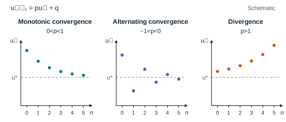
1. Plot of Terms Versus Time Index
Plot on the horizontal axis and on the vertical axis as individual points. Do not join them with a continuous line, as the system only exists at whole-number steps. A sequence flattening towards a horizontal line indicates convergence to a stable equilibrium; points alternating above and below a level line reveal oscillation; points curving outward show divergence.
2. Staircase and Cobweb Diagrams
For any first-order relation , sketch the curve and the diagonal line on the same axes. The intersection where identifies the equilibrium .
To trace the sequence from an initial value on the horizontal axis:
- Move vertically to the curve ; the vertical height is .
- Move horizontally to the diagonal line ; this shifts the value onto the horizontal coordinate.
- Move vertically back to the curve to find , and continue the process.
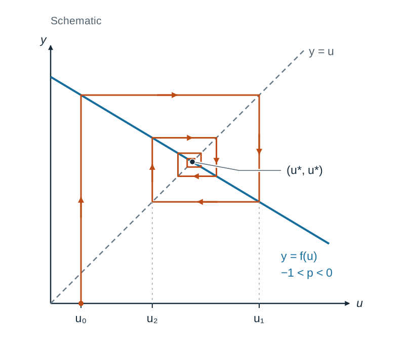
If the curve has a slope between and at the crossing point, the steps spiral or step inwards towards (a stable equilibrium). If the magnitude of the slope exceeds 1, the path moves away (an unstable equilibrium).
In agricultural economics, current supply depends on the previous season's price (), while demand depends on current price (). Equating produces the cobweb model:
Because the slope is negative, the path forms a rectangular spiral around the equilibrium . The market converges if (supply is less sensitive to price changes than demand).
Interpreting and Criticising Models
Exam questions routinely ask you to evaluate your model. Address these three areas:
- Meaning: State what the numbers predict in context with units (e.g. 'predicts 8,110 animals after 10 years').
- Assumptions: Identify assumptions made to create the model (such as a constant growth rate, unchanging repayment terms, or a closed population without migration).
- Limitations: Note where the model breaks down. Linear models with predict infinite growth, which is impossible in a finite environment; a logistic model with a carrying capacity provides a more realistic long-term model.
Key terms
- difference equation
- An algebraic relation linking the terms of a sequence at discrete intervals, expressing future values in terms of one or more previous values.
- order
- The difference between the highest and lowest subscripts of the sequence variable appearing in a difference equation.
- linear
- A difference equation where all sequence terms appear to the first power, are not multiplied together, and do not sit inside non-linear functions.
- non-linear
- A difference equation containing products, powers, or non-linear functions of sequence terms, such as products or squared terms.
- homogeneous
- A difference equation where, after collecting all terms containing the sequence variable on one side, the opposite side is zero.
- inhomogeneous
- A difference equation that contains a non-zero forcing term (constant, polynomial in n, or exponential) independent of the sequence variable.
- first difference
- The change between consecutive terms of a sequence, given by Δu_n = u_(n+1) - u_n.
- second difference
- The difference between consecutive first differences, given by Δ²u_n = u_(n+2) - 2u_(n+1) + u_n.
- characteristic equation
- The quadratic equation a r^2 + b r + c = 0 formed from a second-order linear homogeneous difference equation, whose roots determine the complementary solution.
- complementary solution
- The general solution to the associated homogeneous equation obtained by setting any external forcing terms to zero.
- particular solution
- A specific sequence satisfying the complete inhomogeneous difference equation, matching the mathematical form of the forcing term.
- equilibrium value
- A constant steady-state value u such that if u_n = u, then u_(n+1) = u for all future steps; for u_(n+1) = p u_n + q, u = q / (1 - p).
- stable
- An equilibrium state that the sequence converges toward over time, which occurs in first-order linear models when the multiplier satisfies |p| < 1.
- unstable
- An equilibrium state that the sequence moves away from over time, occurring in first-order linear models when |p| > 1.
- carrying capacity
- The maximum sustainable population size K that an environment can support in a restricted growth model.
- cobweb model
- An economic recurrence model where supply responds to prior prices and demand responds to current prices, generating stepped or spiralling price paths around equilibrium.
Check yourself
What is the characteristic equation and roots for u_(n+2) - 5u_(n+1) - 14u_n = 0?
The characteristic equation is r^2 - 5r - 14 = 0, which factorises as (r - 7)(r + 2) = 0. The roots are r = 7 and r = -2.
Find the equilibrium value of u_(n+1) = 0.75u_n + 25, and determine whether it is stable.
Set u = 0.75u + 25, giving 0.25u = 25, so u = 100. Because |p| = 0.75 < 1, the equilibrium is stable and the sequence converges to 100 as n tends to infinity.
A sequence begins 3, 8, 17, 30, 47. Calculate its first and second differences, and classify the sequence type.
First differences: 5, 9, 13, 17. Second differences: 4, 4, 4. Because the second differences are constant (+4), the sequence is quadratic.
State the trial form for the particular solution of u_(n+2) - 4u_(n+1) + 4u_n = 3(2)^n.
The characteristic equation is (r - 2)^2 = 0, so r = 2 is a repeated root. Because 2^n and n(2)^n already appear in the complementary solution, the trial particular solution is u_n^(p) = C n^2 (2)^n.
In the supply and demand cobweb model P_n = -0.4 P_(n-1) + 42, describe how price behaves over time.
Because p = -0.4 is negative, prices oscillate around the equilibrium. Because |-0.4| < 1, the oscillations dampen and converge to P* = 42 / (1 - (-0.4)) = 42 / 1.4 = 30.
Iterate x_(n+1) = 0.5 x_n (4 - x_n / 10) starting from x_0 = 10 for three steps, and describe what is happening.
x_1 = 0.5(10)(4 - 1) = 15; x_2 = 0.5(15)(4 - 1.5) = 18.75; x_3 = 0.5(18.75)(4 - 1.875) = 19.92. The values are increasing with shrinking increments, converging towards the non-zero equilibrium x* = 20.