
Strand 2 of Leaving Certificate Applied Mathematics models real-world connectivity, logistics, and resource management using networks and graphs. At Higher Level, this strand covers network representations and graph reconstruction, adjacency matrix operations and matrix powers, minimum spanning tree algorithms (Kruskal and Prim), shortest path methods (Dijkstra), multi-stage decision analysis through dynamic programming and Bellman's Principle of Optimality, and project scheduling networks (activity-on-arc networks, dummy activities, critical paths, activity times, and floats).
Network Terminology and Building Models
A network or graph consists of a set of vertices (or nodes) linked by edges (or arcs). When edges carry numerical values like distance, travel time, or laying cost, the network is weighted. If every edge permits travel in only one direction marked by an arrow, the graph is directed (a digraph); if movement is bidirectional, it is undirected.
An undirected graph is connected if you can find a route between every pair of vertices. If any vertex or group of vertices sits isolated, the graph is disconnected. A disconnected graph cannot possess a spanning tree because no set of edges can link all vertices together.
Movement across a network follows precise definitions:
- Walk: A sequence of alternating vertices and edges where both vertices and edges may be repeated (for example, stepping back and forth along the same road).
- Path: A walk in which no vertex is visited more than once.
- Cycle: A closed path that starts and finishes at the same vertex, with no other repeated vertices.
- Tree: A connected undirected graph with no cycles. A tree with vertices always contains exactly edges.
- Spanning tree: A subgraph containing every vertex of the original graph that forms a tree.
The number of edges meeting at a vertex is called its degree. In a simple undirected graph, the degree of a vertex equals the sum of the entries in its row of the adjacency matrix. In a directed graph, we count the two directions separately: a vertex's out-degree is the number of arcs leaving it (its row total in the adjacency matrix) and its in-degree is the number of arcs arriving at it (its column total).
Building a Network from a Scenario
When translating a problem into a network model, determine three elements before drawing:
- Identify the vertices: the distinct entities being joined, such as towns, servers, electrical substations, or project milestones.
- Identify the edges: direct connections between pairs of vertices. Do not add an edge where traffic or signals must pass through an intermediary.
- Identify the weights and units: specify whether weights represent distance in kilometres, transit time in minutes, or capital expenditure in euro.
Assumptions and Limitations
Every network model involves simplifications. In written questions, you are frequently asked to state an underlying assumption and a practical limitation:
- Road distances: we assume link transit times remain constant, whereas actual times fluctuate with weather and rush-hour congestion.
- Utility lines: we assume cables or water pipes run in straight lines at uniform cost per metre, ignoring varied ground terrain, bedrock, and land-access wayleaves.
- Project durations: we assume each activity duration is known with certainty, whereas real tasks face supplier delays and labour shortages.
Adjacency Matrices, Powers, and Graph Reconstruction
An adjacency matrix records the direct connections between vertices in an -vertex graph using an array.
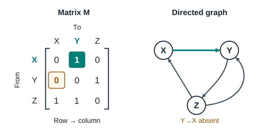
Read an adjacency matrix row first, then column: the entry in row , column records the edges going from vertex to vertex .
- In an unweighted simple graph, the entry if an edge runs from to , and if there is no direct link.
- In an undirected graph, , so the matrix is symmetric across its main diagonal.
- In a directed graph, symmetry generally breaks down because a link from to does not guarantee a link from to .
- When there are no self-loops, the leading diagonal contains only zeros.
Adjacency Matrix versus Distance Matrix
Candidates must distinguish between these two representations:
- An adjacency matrix records how many connections exist (using 0s and 1s, or small integers for parallel edges). Only adjacency matrices can be multiplied to count routes.
- A distance (weight) matrix records how long or costly each direct link is, placing a dash () or where no direct connection exists. You use distance matrices for Prim's tabular method or to read costs. You never multiply a distance matrix; its powers have no mathematical meaning.
Powers of an Adjacency Matrix
Multiplying an adjacency matrix by itself using standard row-by-column matrix multiplication yields a direct count of journeys:
For example, the diagonal entry counts all walks of length 2 from vertex back to itself. In a simple undirected graph, this matches the degree of vertex because each incident edge provides an out-and-back walk ().
If matrix records bus routes and matrix records rail connections across the same ordered hubs, the product entry gives the number of two-stage journeys from to made by taking a bus followed by a train.
Reconstructing a Graph from an Adjacency Matrix
To redraw a network from its matrix:
- Read the dimensions: an matrix contains vertices. Set down labelled nodes in alphabetical or numerical order.
- Test for symmetry: if for all entries, the graph is undirected (draw plain lines). If not symmetric, the graph is directed (draw arrows pointing from row to column ).
- Insert connections: an entry of 1 creates an edge. An entry of creates parallel edges. Non-zero diagonal entries represent loops returning to the same vertex.
Minimum Spanning Trees: Kruskal's and Prim's Algorithms
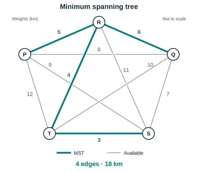
A minimum spanning tree (MST) connects all vertices of a weighted, connected undirected graph using exactly edges while producing the smallest possible sum of edge weights.
Kruskal's Algorithm
Kruskal's algorithm operates globally on the sorted edge list:
- List every edge in the network in ascending order of weight.
- Select the cheapest available edge.
- Add the next cheapest edge, unless it creates a cycle with edges already accepted. If both endpoints already belong to the same connected component, reject the edge and write down the cycle it would close.
- Stop immediately once exactly edges have been accepted.
Prim's Algorithm
Prim's algorithm grows a single tree locally from a designated starting vertex:
- Begin at the specified vertex (or choose any vertex if none is stated).
- Look at all edges connecting any vertex already in the growing tree to any vertex outside the tree.
- Pick the connecting edge with the lowest weight. Add that edge and its new vertex to the tree.
- Repeat until all vertices belong to the tree.
Distance Table Method for Prim
When data appears as a distance matrix rather than a diagram:
- Select the start vertex. Cross out its horizontal row and write label 1 above its vertical column.
- Search all numbered columns for the smallest uncrossed numerical entry.
- Circle this minimum number, identify its row vertex, write the next sequential number above that vertex's column, and cross out its row.
- Search all numbered columns again for the lowest uncrossed weight. Repeat until every row is crossed out.
Comparing Kruskal and Prim
- Prim expands one unbroken tree. It never forms separate components, so it cannot create cycles and requires no cycle checks. It works well on dense networks and distance matrices.
- Kruskal builds separate fragments that gradually merge. It requires explicit cycle checks on each candidate edge. It is quick to execute by hand on sparse diagrams.
- Justification of correctness: Both are greedy algorithms that guarantee a globally optimal tree. At every step, the cheapest edge spanning the divide between vertices already connected and vertices not yet connected must belong to some minimum spanning tree; substituting any costlier edge across that divide would increase the total weight. Terminating after non-cyclic edges guarantees a connected spanning tree of minimal weight.
Shortest Paths: Dijkstra's Algorithm
Dijkstra's algorithm determines the shortest path from a single source vertex to every other vertex in a weighted network. It requires all edge weights to be non-negative ().
Vertex Labelling Layout
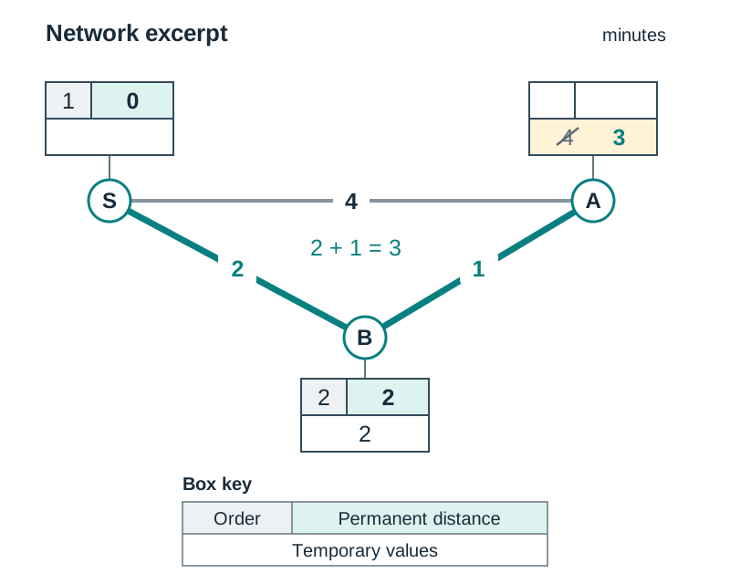
Examiners award method marks for clear working boxes at each vertex. Draw a divided box beside each vertex:
- Order of permanent labelling (top left): 1, 2, 3, ...
- Permanent label (top right): the finalised shortest distance from the source.
- Temporary labels (bottom): working distance values, recorded left to right, with superseded numbers crossed out neatly rather than erased.
Algorithm Procedure
- Set the source vertex permanent label to 0, mark its order as 1, and make all other initial labels empty or .
- From the vertex just made permanent, calculate tentative distances to each unvisited neighbour :
If this candidate distance is smaller than the current temporary label at , write the new value into 's box and score a line through the old value.
- Scan all temporary labels across the entire graph. Select the vertex with the lowest temporary value. Declare this value permanent, write it in the top right, and record the next order number in the top left.
- Repeat steps 2 and 3 until the destination vertex receives its permanent label.
Finding the Route (Back-Tracking)
The permanent labels provide the minimum distance. To recover the sequence of vertices, trace backward from the destination to the source . A preceding vertex sits on the shortest path to if and only if:
Dynamic Programming and Bellman's Principle of Optimality
Dynamic programming breaks multi-stage decision problems into simpler nested sub-problems. It is governed by Bellman's Principle of Optimality:
"An optimal policy has the property that whatever the initial state and initial decision are, the remaining decisions must constitute an optimal policy with regard to the state resulting from the first decision."
In plain English: every piece of a best route, from any point onwards, must itself be a best route from that point. Because dynamic programming evaluates the immediate cost plus the optimal remaining cost, it cannot be deceived by an attractive early step that leads into a costly dead end.
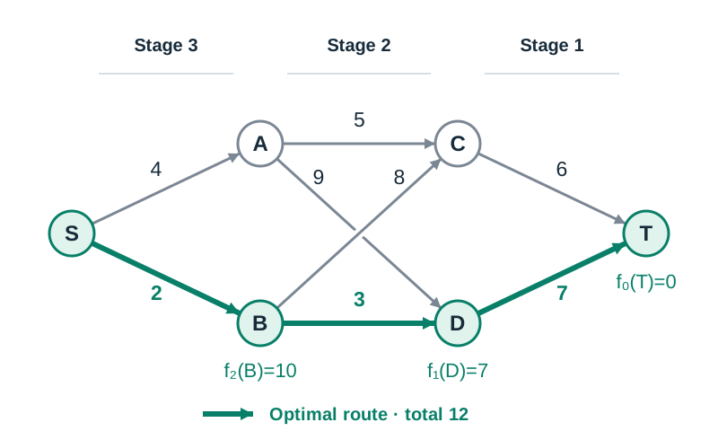
Dynamic Programming Terminology
- Stage (): A step, time interval, or network layer in the decision process, numbered backward from the destination ( is the final transition into the target).
- State (): The specific node, inventory level, or physical condition occupied at the start of a stage.
- Decision (): The next state chosen from state .
- Optimal policy: The complete schedule of optimal decisions from start to finish.
- Optimal value function (): The minimum (or maximum) cumulative return from state to project completion over remaining stages.
Algebraic Recurrence Relation
For finding a shortest route in a weighted directed acyclic network:
where is the immediate cost of stepping from state to state , and is the optimal cumulative cost from state through all subsequent stages.
Required Contexts
The syllabus applies dynamic programming to four authentic problem types:
- Routing: identifying least-cost paths across layered transit zones.
- Stock control: choosing production or reorder quantities to satisfy varying monthly demands while minimising storage charges.
- Allocation of resources: distributing limited funding, machinery, or staff across projects to maximise total return.
- Equipment replacement: deciding whether to keep existing plant (paying higher repair costs) or trade it in for new machinery.
Project Scheduling: Networks, Critical Paths, and Floats
Project management uses activity-on-arc networks. Arrows represent activities with defined durations, while circular nodes represent milestone events marking the completion of incoming activities and the initiation of outgoing ones.
Drawing from a Precedence Table and Dummy Activities
- Begin at a single start event (event 1 at time 0) and draw all activities with no predecessors leaving it.
- An activity can only depart from an event once all its predecessors have arrived there.
- End at a single finish event; any activity with no successor must terminate here.
- Number events sequentially so that every arrow runs from a lower index to a higher index.
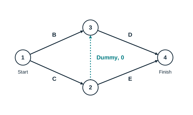
A dummy activity is drawn as a dotted arrow carrying zero duration and consuming no resources. It is required in two circumstances:
- Dependency logic: if activity D requires both B and C to finish, but activity E requires only C, activities B and C cannot run into the same event. Terminate C at its own event, launch E from there, and run a dotted dummy arrow from C's finish event to B's finish event where D starts.
- Unique identification: two parallel activities must not share the same start event and same end event, because activities are referenced by event pairs . Insert a dummy to create a separate milestone.
Forward Pass and Backward Pass
- Earliest event time (EET): Set at the initial event. Moving forward to event :
Take the maximum where arrows converge, because an event cannot occur until every preceding activity finishes.
- Latest event time (LET): Set at the final event. Moving backward to event :
Take the minimum where multiple arrows depart backward, to protect every downstream deadline.
Activity Times and Floats
For an activity of duration :
- Earliest start
- Earliest finish
- Latest finish
- Latest start
Total float measures how long an activity can be delayed without delaying overall project completion:
Free float measures how long an activity can be delayed without delaying the earliest start of any immediate successor:
Critical Path and Sensitivity
The critical path is the longest path from start to finish; its length dictates the minimum total project duration. Activities on this path have zero total float. An activity whose endpoints satisfy is not automatically critical unless its duration matches .
Sensitivity rule: If a non-critical activity is delayed, the overall project duration increases only by the amount by which that delay exceeds the activity's total float. When that happens, recalculate the event times, because the critical path may switch to that activity.
Algorithm Evaluation and Comparison
Higher Level examination questions regularly require students to justify their choice of algorithm or compare alternative methods.
| Algorithm | Paradigm | Primary Objective | Network Requirements |
|---|---|---|---|
| Kruskal | Greedy | Minimum spanning tree | Connected, weighted, undirected graph |
| Prim | Greedy | Minimum spanning tree | Connected, weighted, undirected graph (diagram or distance matrix) |
| Dijkstra | Greedy | Single-source shortest paths | Directed or undirected network with non-negative edge weights () |
| Bellman | Dynamic programming | Multi-stage shortest or longest route | Weighted directed acyclic network divisible into distinct stages |
Evaluating Shortest-Route Techniques
- Exhaustive listing (inspection): Checks every conceivable route. Works reliably on tiny toy graphs, but becomes impossible on real networks because route combinations grow factorially.
- Dijkstra's algorithm: Exceptionally fast. Solves the shortest path from the source to every other vertex simultaneously. However, its greedy logic requires non-negative edge weights. If any weight is negative (such as an incentive, toll refund, or environmental credit), making a label permanent prematurely can return an incorrect path.
- Dynamic programming (Bellman): Evaluates every state across ordered stages. It handles negative transition weights seamlessly and accommodates complex boundary constraints (such as machine capacity, warehouse limits, or fleet turnover cycles). It requires the network to be acyclic so stages cannot loop back on themselves.
Key terms
- Adjacency matrix
- A square matrix where the entry in row i and column j indicates the number of directed edges passing from vertex i to vertex j.
- Walk
- A sequence of alternating vertices and edges connecting an initial vertex to a terminal vertex, in which vertices and edges may be repeated.
- Path
- A walk in which no vertex is visited more than once.
- Cycle
- A closed path starting and ending at the same vertex with no other vertices repeated.
- Tree
- A connected undirected graph that contains no cycles, containing exactly n - 1 edges for n vertices.
- Spanning tree
- A subgraph that contains every vertex of the original graph and forms a tree.
- Minimum spanning tree
- A spanning tree in a weighted undirected graph whose total edge weight is the minimum possible.
- Greedy algorithm
- An algorithm that makes the locally optimal choice at each step without reconsidering earlier choices.
- Bellman's Principle of Optimality
- The principle stating that an optimal policy has the property that whatever the initial state and initial decision are, the remaining decisions must constitute an optimal policy with respect to the state resulting from that first decision.
- Stage
- A distinct step, time period, or network layer in a dynamic programming sequence, conventionally numbered backward from the final objective.
- State
- The condition, location, or parameter value of a system at the beginning of a dynamic programming stage.
- Optimal policy
- The complete sequence of decisions across all stages that achieves the optimum overall payoff or minimum total cost.
- Temporary label
- An interim upper-bound distance assigned to a vertex in Dijkstra's algorithm, subject to reduction when a shorter path is uncovered.
- Permanent label
- A finalised, fixed numerical value in Dijkstra's algorithm representing the confirmed shortest distance from the source vertex.
- Earliest event time
- The earliest time a project milestone event can be reached, calculated during the forward pass by taking the maximum incoming completion time.
- Latest event time
- The latest time an event can take place without delaying overall project completion, calculated during the backward pass by taking the minimum outgoing requirement.
- Critical path
- The continuous path of activities from project start to finish with zero total float, which dictates the minimum duration needed to complete the project.
- Total float
- The amount of time an activity can be delayed from its earliest start without delaying project completion: LET(head) - EET(tail) - duration.
- Free float
- The amount of time an activity can be delayed without delaying the earliest start of any immediate successor: EET(head) - EET(tail) - duration.
- Dummy activity
- An activity of zero duration and zero resource consumption, drawn as a dotted arrow to preserve dependency logic or provide unique identification.
Check yourself
A directed graph with vertices A, B, C has the adjacency matrix: $$ List the edges of this graph, state its in-degrees and out-degrees, and explain whether it contains any cycles.
Reading row to column: the edges are A → B, A → C, and B → C. Vertex A has out-degree 2 and in-degree 0; B has out-degree 1 and in-degree 1; C has out-degree 0 and in-degree 2. All arcs move strictly forward (A to B to C), so the graph contains no cycles (it is acyclic).
A connected network contains 8 vertices. How many edges must be accepted to form a minimum spanning tree, and can the algorithm create a cycle?
A spanning tree on n vertices always contains exactly n - 1 edges, so it requires 8 - 1 = 7 edges. An MST is a tree, so by definition it cannot contain any cycles.
Why does Dijkstra's algorithm fail if a network contains negative edge weights?
Dijkstra is a greedy algorithm that permanently fixes the shortest tentative label found so far, assuming subsequent steps can only add non-negative distance. A negative edge encountered later could produce a shorter route to an already permanent vertex, invalidating the optimality guarantee.
Activity K has a duration of 5 days, starts at an event with EET = 6 and LET = 7, and ends at an event with EET = 14 and LET = 16. Calculate its earliest start, latest finish, total float, and free float.
Earliest start = EET(tail) = 6. Latest finish = LET(head) = 16. Total float = LET(head) - EET(tail) - duration = 16 - 6 - 5 = 5 days. Free float = EET(head) - EET(tail) - duration = 14 - 6 - 5 = 3 days.