

The mathematical modelling project accounts for 20% of Leaving Certificate Applied Mathematics (100 marks out of 500 total), while the terminal written examination accounts for the remaining 80% (400 marks). Completed in sixth year over no more than 20 hours of in-school time, the project requires you to investigate an authentic, open-ended scenario set by an annual State Examinations Commission (SEC) brief. For the 2027 examination cohort, the brief issues to schools in November 2026. The task and assessment criteria are identical for Ordinary Level and Higher Level; differentiation occurs through separate marking schemes applied once your examination level is confirmed. At Ordinary Level, students select from a range of models and apply known solutions to familiar and unfamiliar contexts. At Higher Level, students are expected to select from a range of models and build models from fundamental principles, engaging with theoretical concepts and abstract thinking with significant depth. Sensitivity analysis, validation, and iteration belong to the high-achievement column at both levels; Higher Level candidates demonstrate them with greater mathematical depth and rigour.
The Project Framework, Calendar, and Regulations
Applied Mathematics assesses course content and skills through two complementary modes: a terminal written examination and a digital modelling project report. The project assesses course content and skills that cannot easily be assessed by the written examination, giving you ownership of decisions across the entire modelling cycle.
Key Dates for the Project (2027 Cohort)
- The SEC issues the common brief to schools in November 2026, roughly four weeks earlier than normal under current senior cycle arrangements.
- The completion date for submitting the digital report falls close to the February mid-term break of sixth year. The exact date is fixed by an SEC circular; confirm this date with your teacher when the brief arrives.
- All work must be completed within no more than 20 hours of in-school time in sixth year under teacher supervision.
Practical Allocation of Your 20 In-School Hours
Because 20 hours across ten to twelve weeks passes quickly, pacing is vital. A practical breakdown is:
- Hours 1–4: Read the brief, carry out background research, and fix a precise problem statement.
- Hours 5–8: Identify variables and parameters, state assumptions with justifications, and build Model 1.
- Hours 9–12: Compute solutions, implement spreadsheet formulas or code, and tabulate results.
- Hours 13–16: Validate against real data, test parameter sensitivity, and build Model 2 to iterate the process.
- Hours 17–20: Write conclusions, verify citations, check graphical standards, and format the official booklet.
A student who spends twelve hours researching risks running out of time for sensitivity analysis and iteration, which sit in the high-achievement band.
Authenticity, Supervision, and Digital Presentation
The report must be your own original work submitted in the official SEC digital completion booklet. Your teacher's role is to clarify requirements, prompt critical thinking, provide resources, and manage deadlines. It is not envisaged that your teacher will edit draft reports or provide model text or answers for you to use. Full references and bibliographic citations are required for external formulas, datasets, and code. All media must comply with your school's Acceptable Use Policy, Data Protection Policy, and GDPR. Photographs of identifiable individuals must not be included without written permission.
Do not try to pre-build a finished model before November 2026. Because the 2027 theme is unknown until released, the best preparation is to practice the four-step cycle on familiar situations so the habit of justifying assumptions and testing sensitivity becomes second nature.
Modelling Problems versus Word Problems: Building Models at Higher Level
The specification makes a clear distinction between two types of mathematical tasks:
- A word problem explicitly states all necessary numerical data. You select a known formula and compute one predetermined answer.
- A modelling problem is messy and open-ended, and nothing is scripted for you. You must research, measure, or estimate quantities yourself. You decide which factors matter, simplify the system through assumptions, and construct a mathematical model that gives a useful insight into the situation.
At Higher Level, you are expected to build and adapt models using syllabus concepts across Strands 2, 3, and 4:
- Differential and Difference Equations: Setting up continuous models using Newton's laws with resistive forces () or establishing discrete recurrence relations () to model populations, financial balances, or queues.
- Kinematics and Mechanics: Resolving forces, applying energy conservation, and accounting for friction and mechanical delays.
- Networks and Algorithms: Formulating multi-stage optimisation problems using dynamic programming, critical path analysis, or shortest-path algorithms.
Assumptions versus Approximations
Models rely on two different kinds of simplification:
- An assumption alters the structure of the model by deciding which terms and physical effects enter your equations. For example, assuming a track is level or assuming air resistance is negligible.
- An approximation alters the precision of a numerical input fed into those equations. For example, using , rounding a measured reaction time to 0.8 s, or taking an average service rate from a sample of timings.
You critique an assumption by removing it or refining its mathematical form; that is model iteration. You test an approximation by measuring how much the calculated answer shifts when the value moves across its plausible range; that is sensitivity analysis.
Stage 1: Formulating the Problem and Selecting Variables
Formulation turns a broad theme into a clear, solvable mathematical inquiry. The high-achievement criterion requires you to state the problem concisely, early in the written report. Aim for a single, prominent sentence on your opening page that specifies the exact mathematical output, units of measure, constraints, and your perspective as a modeller.
Real situations contain dozens of influencing factors. Through abstraction, you isolate the primary components and set aside secondary details.
Identifying and Justifying the Dominant Factor
Do not simply list variables. The marking criteria require you to identify several variables and justify the need for the main factor influencing the phenomenon. State which factor dominates and why other factors can be neglected. For example:
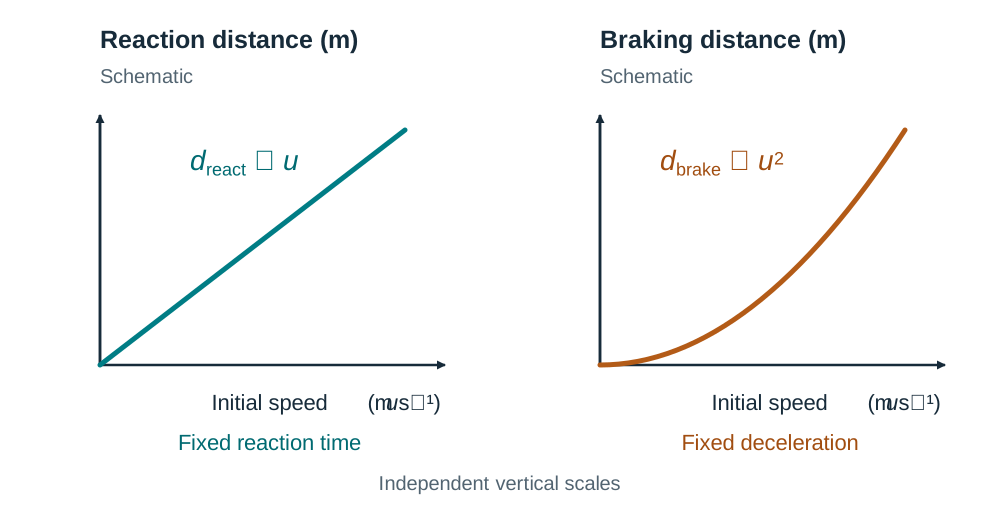
"Of these variables, initial speed is the dominant factor. Reaction distance increases linearly with , while mechanical braking distance increases with . At operating speeds, a 20% increase in speed adds roughly 40% to braking distance but only 20% to reaction distance. Deceleration ranks next. Rider mass has negligible influence: for a rolling or skidding tyre, the retarding friction force is , giving , which is independent of mass. Mass is therefore excluded from the model."
Writing Defensible Assumptions
Listing assumptions without explanation places a project in the moderate or low achievement bands. To achieve the top band, every assumption requires a real-world justification and an explicit limitation.
| Real-World System | Simplifying Assumption | Justification | Stated Limitation |
|---|---|---|---|
| Vehicle Stopping Distance | Deceleration is constant during mechanical braking. | Anti-lock brakes on dry tarmac maintain a reasonably stable coefficient of friction . | Ignores hydraulic pressure build-up and thermal brake fade during prolonged braking. |
| Domestic Rainwater Catchment | The roof catchment area is a flat, horizontal two-dimensional plane. | The plan projection represents the horizontal footprint intercepting falling rain. | Ignores splash losses from high winds and gutter overflow during intense downpours. |
| School Canteen Queuing | Service time per student is constant across checkout tills. | Sample measurements show transaction times cluster closely around a mean duration. | Fails to capture delays caused by card machine signal drops or complex custom food orders. |
Criteria marked against in this stage: Problem Statement; Assumptions and Variables.
Stage 2 and Stage 3: Translating to Mathematics and Computing Solutions
Translation converts your assumptions and variables into mathematical notation. A variable changes value across states or over time (), while a parameter remains fixed during a single computational run but can be changed between runs to test different conditions (such as reaction delay or friction coefficient ).
You must explain the relationship between wholes and parts by breaking complex systems into linked mathematical sub-problems. In stopping distance, the whole distance is the sum of two distinct parts: reaction distance and braking distance ().
Creating Computer-Interpretable Models
The specification requires students to create a mathematical model that can be interpreted by a computer and use computational technology to solve problems. Standard digital tools include:
- Spreadsheets: Implementing discrete difference equations and recurrence models where changing an input cell recalculates the entire output sequence.
- Programming code: Writing Python or R scripts to execute numerical algorithms or multi-step simulations.
- Graphing software: Plotting functions and rate equations in GeoGebra or Desmos to visualise turning points and intersections.
The assessment criteria reward clear insight and logical mathematical reasoning into the method used. A screenshot on its own shows an output, not reasoning. Always write the governing equation or recurrence relation beside any spreadsheet or code output, and explain in one sentence what the computational tool is calculating.
Criteria marked against in this stage: Mathematical Method; Solution and Presentation.
Stage 4: Evaluating, Validating, Sensitivity Testing, and Iterating
Finding a numerical answer does not mean your model works. In Stage 4, you assess the reliability of your model using four systematic checks.
1. Plausibility and Graph Behaviour
Begin with basic sign and magnitude checks (times and queue lengths cannot be negative). Then interrogate the shape of your model's graph:
- Intercepts: Check what happens at or . A stopping-distance model must yield when ; if it yields a positive distance, stationary vehicles are being assigned a stopping delay.
- Turning points: Do maximum or minimum values occur at realistic times, and are their magnitudes physically possible?
- Long-term behaviour: What happens as the independent variable grows large? A queue model predicting negative customers or a population model growing infinitely large indicates that the model has been pushed beyond its valid limits.
- Systematic graphical trends: When plotting model curves against real data points, note whether the model consistently overestimates or underestimates values at the extremes. A systematic divergence highlights which assumption to adjust.
2. Quantitative Model Validation
Compare your mathematical predictions directly against an independent benchmark, such as published technical data, road safety figures, or timed field experiments. Measure accuracy using percentage error:
In your submitted booklet, this benchmark must be a genuine, fully cited figure; benchmarking against an estimated number carries no validation credit.
3. Sensitivity Analysis: Robust versus Fragile
Test how your model responds when input parameters vary within their realistic range of uncertainty. A perturbation of 10% to 25% should be justified by context (for instance, tyre friction drops by roughly 25% on wet asphalt):
- If a 20% change in an input produces a 3% change in output, the model is robust regarding that parameter.
- If a 20% change in an input causes a 60% swing in output, the model is fragile, meaning the real-world decision depends heavily on that estimate.
4. Demonstrating Model Iteration
Iteration separates the high achievement band from the moderate band. The criteria require that the model is refined and the process iterated. When Model 1 shows discrepancies during validation, return to earlier stages: refine an assumption, introduce an omitted physical factor, re-solve the system as Model 2, and prove that the percentage error has decreased.
Criteria marked against in this stage: Evaluation and Iteration.
Report Structure, Marking Criteria, and Submission Self-Check
Your report must be organised according to the structure in Table 3 of the NCCA guidance:
- Introduction and Research: Background context, citations, clear problem statement, identified variables, and baseline data.
- The Modelling Process: Justified assumptions, mathematical formulation, computational steps, labelled graphs, sensitivity tests, and documented iteration (Model 1 compared with Model 2).
- Interpretation of Results: Real-world meaning of numbers, clear recommendations, and reflections on limitations.
- Communication and Innovation: Assessed holistically across the report for readability, professional layout, correct units, and creative problem-solving.
SEC Modelling Project Assessment Criteria
| Assessment Category | High Level of Achievement | Moderate Level of Achievement | Low Level of Achievement |
|---|---|---|---|
| Problem Statement | States problem statement concisely, early in written report. References sources. | Problem statement not precise or inconsistent with other statements. | Problem statement difficult to understand or buried in text. |
| Assumptions & Variables | Identifies several variables; justifies dominant factor; justifies assumptions with limitations. | Lists parameters and variables without sufficient explanation; notes assumptions without justification. | Assumptions identified and justified, but reader cannot locate them; variables barely mentioned or hard to find. |
| Mathematical Method | Clear insight with logical mathematical reasoning into methods; plausible approach and outcome. | Stated approach contains aspects that are inconsistent, difficult to understand, or incomplete. | States a model, but it contains fixable mathematical errors. |
| Solution & Presentation | Accurately-computed solution; clear relationship between variables; consistent visual aids and units. | Answer stated, but lacks context, omits units, or features unclear visual aids. | States an answer without contextual background or units; or arrives at no solution. |
| Evaluation & Iteration | Addresses viability; thorough sensitivity analysis; compares to data; model refined and iterated. | Addresses viability, but analysis lacks proper dimensionality; obvious consequences ignored; no iteration. | Provides some analysis without perspective; uses incorrect mathematics in analysis. |
| Communication | Paper is well-formatted, enjoyable to read, with easy-to-interpret visual aids. | Multiple spelling, formatting, or grammatical errors; visual aids missing key readability features. | Significant disregard for common spelling, grammatical, and mathematical rules. |
Note the descriptor in the low band for mathematical method: states a model, but it contains fixable mathematical errors. A calculation slip inside an otherwise sound method does not drop a report to the low band; omitting mathematical reasoning entirely is what drops it. In assumptions, the moderate band lacks justification, while the low band lacks clear signposting. Both are avoided by using a clearly headed table near the start.
Four-Line Self-Check Before Submission
The specification states that the project requires students to demonstrate four core capabilities. Check that you can point to specific pages for each:
- Define a problem: Is there one clear sentence early on stating exactly what output or decision my model produces?
- Translate the problem to mathematics: Are variables, parameters, and units defined, and are governing equations written down?
- Compute a solution: Are computational steps shown with units, and is the answer interpreted in the real situation?
- Analyse the solution and iterate the process: Did I test the model, identify a weakness, and adjust the model based on the result?
Key terms
- Modelling Problem
- An open-ended investigation requiring the solver to research the situation, make reasonable assumptions, determine relevant variables, and build a mathematical model that best describes the context.
- Word Problem
- A closed exercise explicitly providing all necessary information, requiring only the selection of an established procedure to compute a single predetermined correct answer.
- Problem Statement
- A concise, unambiguous declaration placed early in the report specifying the exact mathematical output, units, scope, and perspective of the investigation.
- Abstraction
- The process of isolating essential governing relationships and features within a real-world system while deliberately setting aside minor, non-essential details.
- Assumption
- A structural simplification made to real-world conditions to make mathematical analysis tractable; requires explicit justification and a stated limitation.
- Approximation
- A simplification affecting the numerical precision of a parameter, measured value, or constant used as an input to a model.
- Variable
- A measurable quantity that changes continuously or takes different values across states during an investigation, such as time, speed, or queue length.
- Parameter
- A quantity held fixed during a specific calculation run of a model but adjustable across different scenarios to investigate model sensitivity.
- Validation
- The process of testing model viability and accuracy by comparing mathematical predictions against independent empirical measurements, manufacturer specifications, or published data.
- Sensitivity Analysis
- The systematic adjustment of key input parameters or assumptions across plausible ranges to observe the percentage change in output, determining whether the model is robust or fragile.
- Robust
- A model characteristic where substantial shifts in an input parameter or assumption produce only minor, acceptable variations in the computed output.
- Fragile
- A model characteristic where small adjustments to an input parameter or assumption cause disproportionately large swings in the calculated outcome.
- Model Iteration
- The process of evaluating an initial model against evidence, identifying structural simplifications that compromise accuracy, and reforming the mathematics into an improved subsequent model.
- Common Brief
- The official assignment document issued annually by the State Examinations Commission containing the authentic scenario and submission instructions common to both Higher and Ordinary Level.
- Critical Path
- The longest path through an activity network that determines the minimum project duration, where every activity has zero float and early event times equal late event times.
- Zero Float
- A condition in project scheduling where an activity's earliest start time and latest finish time leave no spare scheduling slack, meaning any delay directly delays the overall project.
Check yourself
What proportion of Leaving Certificate Applied Mathematics marks is allocated to the modelling project, and what is the maximum in-school time permitted?
The project accounts for 20% (100 marks out of 500 total) and must be completed in no more than 20 hours of in-school time in sixth year.
An SEC brief asks you to investigate 'the efficiency of the school bus service'. Write a problem statement that satisfies the high-achievement assessment criterion.
'To determine the minimum number of pick-up stops along the Ballyroan route that allows all 54 registered students to arrive at the school gate by 08:50, from the perspective of the transport co-ordinator, assuming an average dwell time of 25 s per stop.'
Increasing an assumed reaction time from 0.8 s to 0.9 s (a 12.5% increase) changes a model's predicted stopping distance from 9.83 m to 10.39 m. Is the model robust or fragile with respect to reaction time?
The output changes by (10.39 - 9.83)/9.83 * 100% = 5.7%. Because a 12.5% change in parameter produces only a 5.7% change in stopping distance, the model is robust with respect to reaction time.
What is the structural difference between an assumption and an approximation in a mathematical model?
An assumption changes the structure of the model by deciding which terms and physical effects enter the equations, while an approximation changes the numerical precision of a parameter or measured input.
What are the four official core capabilities the modelling project requires students to demonstrate?
1. Define a problem; 2. Translate the problem to mathematics; 3. Compute a solution; 4. Analyse the solution and iterate the process.
State the formula used to calculate absolute percentage error when validating a model against a benchmark.
Percentage Error = (|Predicted Value - Observed Benchmark| / Observed Benchmark) * 100%.