Integration

Standard Forms and Integration by Substitution

The standard integrals you need are supplied in the Formulae and Tables booklet. The core exam skill is recognising which standard form an expression matches.

The power rule integrates any variable raised to a constant real power other than $-1$:

The power rule fails when $n = -1$, because it would require division by $n + 1 = 0$. That case has its own standard result, giving the natural logarithm:

For a linear denominator, dividing by the inner derivative gives:

Other essential standard forms include:

• $\int e^{kx} \, dx = \frac{1}{k}e^{kx} + c$
• $\int \cos(kx) \, dx = \frac{1}{k}\sin(kx) + c$
• $\int \sin(kx) \, dx = -\frac{1}{k}\cos(kx) + c$
• $\int \frac{1}{x^2 + a^2} \, dx = \frac{1}{a}\tan^{-1}\left(\frac{x}{a}\right) + c$
• $\int \frac{1}{\sqrt{a^2 - x^2}} \, dx = \sin^{-1}\left(\frac{x}{a}\right) + c$

Integration by substitution reverses the chain rule of differentiation. It is used when an integrand contains an inner function $g(x)$ multiplied by a scalar multiple of its derivative $g'(x)$:

For definite integrals, convert the limits of integration to values of $u$ immediately rather than converting back to $x$ at the end. For example, to evaluate $\int_0^2 \frac{v}{v^2 + 4}\,dv$, let $u = v^2 + 4$, giving $du = 2v\,dv$, so $v\,dv = \frac{1}{2}du$. When $v = 0$, $u = 4$; when $v = 2$, $u = 8$:

A fast self-check habit: differentiate your final integrated expression. If you do not recover the original integrand, you have made a slip with a constant or a sign.

Integration by Parts

When an integrand is a product of two distinct families of functions that substitution cannot resolve, use integration by parts. The formula comes directly from integrating the product rule of differentiation:

To choose which part to differentiate as $u$ and which to integrate as $dv$, use the ILATE rule of thumb. Prioritise $u$ in this order:

• I: Inverse trigonometric (such as $\tan^{-1}x$, $\sin^{-1}x$)
• L: Logarithmic (such as $\ln x$)
• A: Algebraic (such as $t$, $3x^2$, $x + 1$)
• T: Trigonometric (such as $\sin(kx)$, $\cos(kx)$)
• E: Exponential (such as $e^{kx}$, $e^{-2t}$)

Assign $u$ to whichever factor appears earlier in ILATE; the rest of the integrand becomes $dv$. Note that ILATE is a mnemonic to guide your choice, not a syllabus theorem to quote for marks; marks are awarded for applying $\int u\,dv = uv - \int v\,du$ correctly.

Set out your working clearly:

For a solitary logarithm like $\int \ln(x)\,dx$, treat the integrand as a product with 1: set $u = \ln(x)$ and $dv = 1\,dx$, giving $du = \frac{1}{x}\,dx$ and $v = x$:

Kinematics: The Fundamental Theorem, Graphs, and Deriving Formulae

Velocity is the time derivative of displacement, $v = \frac{ds}{dt}$, and acceleration is the time derivative of velocity, $a = \frac{dv}{dt}$. Integration reverses these operations. When acceleration or velocity varies continuously with time, integrating with respect to $t$ reconstructs the motion functions:

The Fundamental Theorem of Calculus and Area Under Curves

If $F$ is an antiderivative of $f$ such that $F'(t) = f(t)$, the Fundamental Theorem of Calculus states:

Summing the rate of change over an interval yields the net change in that quantity:

• The area under a velocity–time graph between $t_1$ and $t_2$ represents the change in displacement (the Riemann integral): $\Delta s = \int_{t_1}^{t_2} v(t)\,dt$.
• The area under an acceleration–time graph gives the change in velocity: $\Delta v = \int_{t_1}^{t_2} a(t)\,dt = v(t_2) - v(t_1)$.

Areas below the time axis are negative. Displacement measures net change in position, while total distance measures actual ground covered.

Worked Example: Displacement versus Total Distance

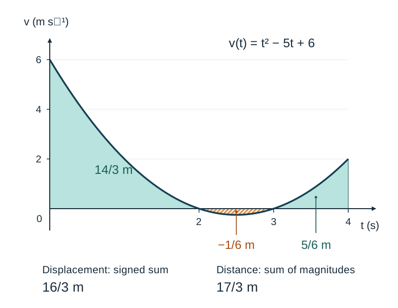
A particle moves in a straight line with $v(t) = t^2 - 5t + 6\,\text{m s}^{-1}$ for $0 \le t \le 4\,\text{s}$.

1. Net displacement over the 4 seconds:

1. Total distance travelled requires finding where velocity changes sign:

Velocity changes sign at $t = 2\,\text{s}$ and $t = 3\,\text{s}$. Split the integral across these intervals and sum their absolute values:

• From $t = 0$ to $t = 2$: $\int_0^2 v\,dt = \Big[\frac{t^3}{3} - \frac{5t^2}{2} + 6t\Big]_0^2 = \frac{8}{3} - 10 + 12 = \frac{14}{3} \approx 4.67\,\text{m}$
• From $t = 2$ to $t = 3$: $\int_2^3 v\,dt = \left(\frac{27}{3} - \frac{45}{2} + 18\right) - \frac{14}{3} = \frac{9}{2} - \frac{14}{3} = -\frac{1}{6} \approx -0.17\,\text{m}$
• From $t = 3$ to $t = 4$: $\int_3^4 v\,dt = \frac{16}{3} - \frac{9}{2} = \frac{5}{6} \approx 0.83\,\text{m}$

Deriving the Kinematic Formulae Using Calculus

When acceleration $a$ is constant, calculus derives the three standard formulae directly:

1. Integrating acceleration with respect to time:

1. Substituting $v = \frac{ds}{dt}$ and integrating again:

1. Connecting acceleration directly to displacement via the chain rule, $a = \frac{dv}{dt} = \frac{dv}{ds}\frac{ds}{dt} = v\frac{dv}{ds}$:

Work, Energy, Impulse, and Variable Forces

For a constant force along the line of motion, work is force multiplied by displacement ($W = Fs$). When force varies with position $x$, we integrate the force function:

Gravity and the Constant-Acceleration Approximation

Lifting a mass $m$ through height $h$ near the Earth's surface opposes a constant force $mg$:

This gives gravitational potential energy. It holds strictly under the constant acceleration approximation ($g = 9.8\,\text{m s}^{-2}$). If gravity varied with altitude, $g(r)$ would have to be integrated over distance.

Hooke's Law: Elastic Strings versus Springs

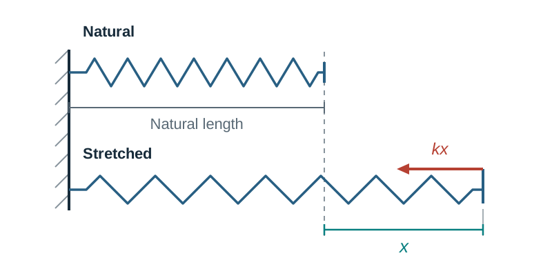
Under Hooke's Law, the restoring force has magnitude $F = kx$, where $x$ is the extension or compression beyond natural length and $k$ is the elastic constant in $\text{N m}^{-1}$.

• An elastic string can only be stretched ($x > 0$). When compressed or at natural length, tension is zero ($T = 0$) because strings go slack; they cannot push.
• A spring can be stretched or compressed. Under compression $x$, it exerts an outward thrust of magnitude $kx$.

Because the restoring force opposes displacement, it acts as $-kx$ when writing an equation of motion. The work done in stretching from natural length ($x = 0$) to extension $x$ is stored as elastic potential energy ($E_p$):

When calculating work between extensions $x_1$ and $x_2$, the integral is $\int_{x_1}^{x_2} kx\,dx = \frac{1}{2}kx_2^2 - \frac{1}{2}kx_1^2$. The limits must always be extensions beyond natural length, never the total lengths of the string.

The Work–Energy Theorem

The net work done on a particle equals its change in kinetic energy:

Notice that the limits switch from positions ($x_1, x_2$) to velocities ($u, v$) the moment the differential changes from $dx$ to $dv$.

Impulse of a Variable Force

For a constant force, impulse is $I = Ft$. When force varies with time, impulse is the integral of force over time, which equals the change in linear momentum:

For example, if a force $F(t) = 300t(0.1 - t)\,\text{N}$ acts on a $0.5\,\text{kg}$ ball initially at rest for $0.1\,\text{s}$:

First-Order Separable Differential Equations in Resisted Motion

When resistance depends on velocity—such as fluid drag or aerodynamic resistance proportional to $v^n$ ($n \in \mathbb{R}$)—Newton's Second Law produces a differential equation. Setting up the equation requires choosing the correct calculus form for acceleration:

• If the problem connects velocity and time, use $a = \frac{dv}{dt}$.
• If the problem connects velocity and displacement, use $a = v\frac{dv}{ds}$.

Executing a "Show That" Differential Equation Setup

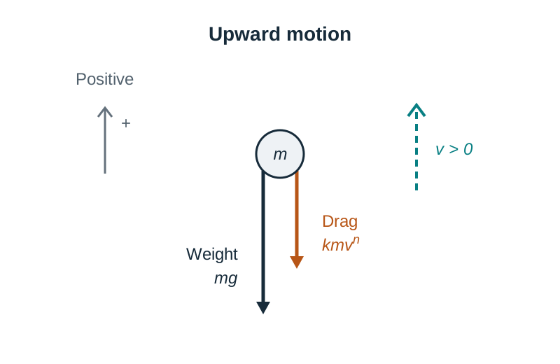
Questions frequently ask you to show that motion satisfies a specific differential equation before asking you to solve it. Marks are awarded for each line of the setup:

1. State the chosen positive direction clearly and list all forces.
2. Write Newton's Second Law with signed forces: for upward motion against gravity and drag, $-mg - kmv^n = ma$.
3. Cancel mass $m$ explicitly (note that $m$ cancels because resistance is given per unit mass; if resistance is given in newtons as $Rv^n$, divide across by $m$ to get $a = -g - \frac{R}{m}v^n$).
4. Replace $a$ with $\frac{dv}{dt}$ or $v\frac{dv}{ds}$, guided by whether the target printed equation contains $t$ or $s$.
5. Rearrange algebraically until your line matches the printed equation exactly, then write "as required".

Solving by Separation of Variables

1. Get everything involving $v$ (including $dv$) on one side and everything involving $t$ or $s$ (including $dt$ or $ds$) on the other. Ensure $dv$, $dt$, and $ds$ end up in numerators, never in denominators.
2. Place matching limits directly on the integral signs, or integrate with an arbitrary constant $+ c$ and evaluate $c$ using initial conditions.
3. Integrate using logarithmic, power, or inverse tangent rules.
4. Rearrange algebraically to make the target variable the subject.

Reducible Second-Order Equations and Continuous Change Models

Second-order differential equations contain second derivatives such as $\frac{d^2s}{dt^2}$ or $\frac{d^2y}{dx^2}$. At Higher Level, equations where either the position variable or the time variable is absent from the right-hand side can be reduced to first order.

Choose the substitution to match the variable appearing in the equation:

• If the equation involves $t$ alongside the derivative (for example, $\frac{d^2s}{dt^2} = -4\frac{ds}{dt}$), write $\frac{ds}{dt} = v$ and $\frac{d^2s}{dt^2} = \frac{dv}{dt}$. This gives $\frac{dv}{dt} = -4v$, which separates directly in terms of $v$ and $t$.
• If the equation involves displacement $s$ (for example, $\frac{d^2s}{dt^2} = -9s$), write $\frac{d^2s}{dt^2} = v\frac{dv}{ds}$. This gives $v\frac{dv}{ds} = -9s$, which separates directly in terms of $v$ and $s$.

After solving the first-order equation for $v$, replace $v$ with $\frac{ds}{dt}$ and integrate a second time to find position $s(t)$.

Continuous Change in Non-Mechanical Systems (Strand 4)

• Malthusian Growth and Decay: The rate of change is proportional to the current quantity: $\frac{dN}{dt} = kN$. Separating variables yields $\int \frac{1}{N}\,dN = \int k\,dt \implies N(t) = N_0 e^{kt}$. When $k > 0$, the model represents exponential growth; when $k < 0$, it models exponential decay. $N_0$ is the quantity present at $t = 0$.
• Newton's Law of Cooling: The rate of temperature change of a body is proportional to the difference between its temperature $\theta$ and the ambient temperature $\theta_{\text{env}}$: $\frac{d\theta}{dt} = -k(\theta - \theta_{\text{env}})$, where $k > 0$ is the cooling constant in units of $\text{s}^{-1}$. The temperature approaches $\theta_{\text{env}}$ asymptotically as $t \to \infty$.

Numerical and Qualitative Alternatives

While analytical integration is primary, the syllabus notes two non-calculus evaluation methods:

• Numerical step-by-step methods (such as Euler's forward step, $y_{n+1} \approx y_n + h f(x_n, y_n)$ with step size $h$), implemented digitally for equations that cannot be integrated analytically.
• Qualitative graphical methods, where setting $\frac{dy}{dt} = 0$ identifies equilibrium values and the sign of $\frac{dy}{dt}$ determines stability.

Key terms

Fundamental Theorem of Calculus

The theorem stating that if $F'(x) = f(x)$, then $\int_a^b f(x)\,dx = F(b) - F(a)$, linking differentiation and integration to evaluate net accumulation.

Riemann Integral

The definite integral interpreted as the limit of a sum of rectangular areas under a curve, representing signed net displacement on a velocity–time graph.

Integration by Substitution

A technique for evaluating integrals by introducing a new variable $u = g(x)$ to reverse the chain rule of differentiation.

Integration by Parts

A calculus technique derived from the product rule of differentiation, evaluated using $\int u \, dv = uv - \int v \, du$.

ILATE

A mnemonic priority order (Inverse trig, Logarithmic, Algebraic, Trigonometric, Exponential) used to select the component $u$ to differentiate in integration by parts.

Separation of Variables

A technique for solving differential equations by algebraically collecting all terms of one variable on one side and all terms of the other variable on the opposite side before integrating.

Terminal Velocity

The limiting steady velocity reached by a falling object when the resistive drag force equals the driving gravitational force, causing acceleration to become zero.

Hooke's Law

A physical law stating that the restoring force exerted by an elastic spring or string is proportional to its extension beyond natural length: $F = kx$.

Elastic Potential Energy

The energy stored in an elastic body stretched or compressed by an extension $x$ from its natural length, given by $E_p = \frac{1}{2}kx^2$.

Work–Energy Theorem

The principle stating that the work done by the net force acting on a particle equals the change in its kinetic energy: $W_{\text{net}} = \Delta E_k$.