Acceleration

Understanding Acceleration as a Vector

Acceleration measures how quickly velocity changes. In physics, acceleration is defined as the rate of change of velocity with respect to time.

Average acceleration is calculated using the formula:

Where:

• $a$ is acceleration in metres per second squared ($\text{m s}^{-2}$)
• $v$ is final velocity in metres per second ($\text{m s}^{-1}$)
• $u$ is initial velocity in metres per second ($\text{m s}^{-1}$)
• $t$ is the time interval taken in seconds ($\text{s}$)

Units and Dimensions

The unit $\text{m s}^{-2}$ means "metres per second, every second". Checking units across equations helps verify your working:

• In $v = u + at$, both $v$ and $u$ have units of $\text{m s}^{-1}$, while $at$ has units $(\text{m s}^{-2})(\text{s}) = \text{m s}^{-1}$.
• In $s = ut + \frac{1}{2}at^2$, $ut$ gives $(\text{m s}^{-1})(\text{s}) = \text{m}$, and $at^2$ gives $(\text{m s}^{-2})(\text{s}^2) = \text{m}$.
• In $v^2 = u^2 + 2as$, $v^2$ has units $\text{m}^2 \text{s}^{-2}$, and $as$ has units $(\text{m s}^{-2})(\text{m}) = \text{m}^2 \text{s}^{-2}$.

Worked Example: Basic Linear Acceleration

A cyclist speeds up from $4.0\text{ m s}^{-1}$ to $10.0\text{ m s}^{-1}$ in $3.0\text{ s}$. Calculate her acceleration.

Her velocity increases by $2.0\text{ m s}^{-1}$ every second in her direction of motion.

Signs and Deceleration

Because acceleration is a vector, you must set a positive direction at the start of any calculation.

• Deceleration means decreasing speed. It happens whenever the acceleration vector points opposite to the velocity vector.
• A negative sign does not always mean slowing down. If an object travels backwards (negative velocity) and accelerates backwards (negative acceleration), both point in the same direction, so the object speeds up in that reverse direction.
• An object moving at constant speed around a curve accelerates because its direction changes continuously. For example, a car going around a roundabout at a steady $30\text{ km h}^{-1}$ accelerates towards the centre of the circle.

Acceleration and Resultant Force

Newton's second law tells us that a constant resultant force acting on a constant mass produces a constant acceleration:

For example, a car of mass $1200\text{ kg}$ with a forward driving force of $3000\text{ N}$ and total resistive forces of $600\text{ N}$ experiences a net force $F_{\text{net}} = 3000 - 600 = 2400\text{ N}$. Its acceleration is $a = \frac{2400}{1200} = 2.0\text{ m s}^{-2}$. When a trolley glides down a smooth slope tilted at angle $\theta$ to the horizontal, the component of gravity down the incline is $mg\sin\theta$, which produces an acceleration along the slope of $a = g\sin\theta$.

Graphical Analysis: Displacement-Time and Velocity-Time Graphs

Graphs give a visual model of motion along a straight line.

Displacement-Time ($s$-$t$) Graphs

Plotting displacement on the vertical axis against time on the horizontal axis yields the following relationships:

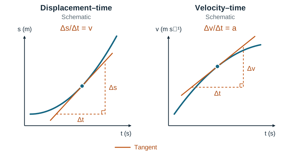
• The slope = velocity ($\text{slope} = \frac{\Delta s}{\Delta t} = v$).
• A horizontal line means the slope is zero, so the object is at rest.
• A straight sloped line indicates constant velocity, meaning zero acceleration.
• A curved line represents changing velocity (acceleration). The instantaneous velocity at any exact point is the slope of the tangent to the curve at that point.

Velocity-Time ($v$-$t$) Graphs

Plotting velocity on the vertical axis against time on the horizontal axis provides both acceleration and spatial progress:

• The slope = acceleration ($\text{slope} = \frac{\Delta v}{\Delta t} = a$).
• A horizontal line represents constant velocity ($a = 0$).
• A straight sloped line represents uniform acceleration.
• A curved line represents varying acceleration. The instantaneous acceleration is the slope of the tangent at that time.
• The area enclosed between the line and the time axis gives position changes:
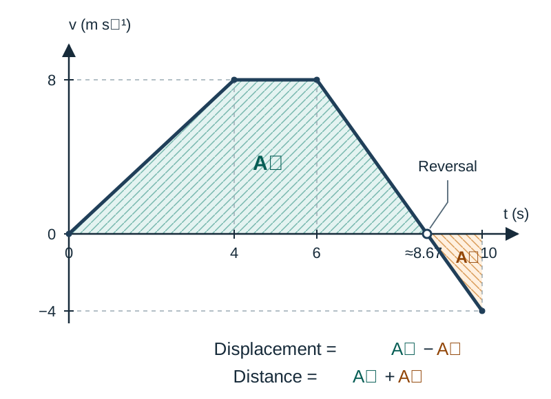
• Displacement = signed area. Any area above the time axis counts as positive displacement, while area below counts as negative displacement:

• Distance = total area. Distance is the total path length travelled and is always positive, so add the absolute values of the areas:

• The magnitude of displacement equals distance travelled only when the body moves in a straight line without reversing.

Worked Example: Velocity-Time Graph with Reversal

A trolley's velocity-time graph has three straight segments:

• From $0\text{ s}$ to $4\text{ s}$, velocity rises steadily from $0$ to $8\text{ m s}^{-1}$.
• From $4\text{ s}$ to $6\text{ s}$, velocity remains at $8\text{ m s}^{-1}$.
• From $6\text{ s}$ to $10\text{ s}$, velocity falls steadily from $8\text{ m s}^{-1}$ to $-4\text{ m s}^{-1}$.

1. Acceleration from $0$ to $4\text{ s}$: $\text{slope} = \frac{8 - 0}{4 - 0} = 2\text{ m s}^{-2}$.
2. Acceleration from $6$ to $10\text{ s}$: $\text{slope} = \frac{-4 - 8}{10 - 6} = \frac{-12}{4} = -3\text{ m s}^{-2}$.
3. Reversal point: the line crosses the time axis ($v = 0$) when dropping $8\text{ m s}^{-1}$ at $3\text{ m s}^{-2}$, taking $\frac{8}{3} \approx 2.67\text{ s}$ after $t = 6\text{ s}$, which is $t \approx 8.67\text{ s}$.
4. Areas:

(using unrounded areas 42.67 m and 2.67 m)

Investigating Varying Motion and Secondary Data

When acceleration changes continuously, the velocity-time graph curves. For example, a falling skydiver experiences increasing air resistance, causing the $v$-$t$ graph to flatten out as the object nears terminal velocity. The slope of the curve gradually falls to zero.

In the laboratory, motion sensors (ultrasonic position sensors) connected to data loggers record displacement dozens of times per second, enabling software to plot instantaneous $s$-$t$ and $v$-$t$ graphs. Secondary data (data recorded by others or provided in tables) can be analysed by reading values, plotting best-fit curves, drawing tangents to measure instantaneous acceleration, and estimating area under curved lines by counting squares or using strip approximations.

Deriving the Kinematic Equations (Higher Level)

Remember: these equations only work when the acceleration is constant. Higher Level candidates are required to derive all three relationships algebraically from first principles.

Derivation 1: $v = u + at$

By definition, acceleration is the rate of change of velocity:

Multiply across by $t$:

Rearranging gives:

Derivation 2: $s = ut + \frac{1}{2}at^2$

Displacement equals average velocity multiplied by time. For constant acceleration, average velocity is the arithmetic mean of initial and final velocity:

Therefore:

Substitute the first equation ($v = u + at$) into this expression:

Separate the terms inside the brackets:

Multiply across by $t$:

(Alternatively, on a $v$-$t$ graph, the total area under the line from $0$ to $t$ forms a trapezium. Splitting it into a lower rectangle of area $ut$ and an upper triangle of height $v - u = at$ and base $t$ gives area $= ut + \frac{1}{2}(t)(at) = ut + \frac{1}{2}at^2$.)

Derivation 3: $v^2 = u^2 + 2as$

Rearrange equation 1 to isolate time $t$:

Substitute this expression into the displacement formula $s = \left(\frac{u + v}{2}\right)t$:

Expand the numerator as the difference of two squares, $(v + u)(v - u) = v^2 - u^2$:

Multiply across by $2a$:

Rearrange to make $v^2$ the subject:

Laboratory Investigations of Linear Acceleration

Physicists investigate linear acceleration experimentally using primary data gathered through standard timing techniques.

Ticker Timer Method

A ticker timer uses an alternating current supply to vibrate an inked pin against paper tape at $50\text{ Hz}$, printing 50 dots each second.

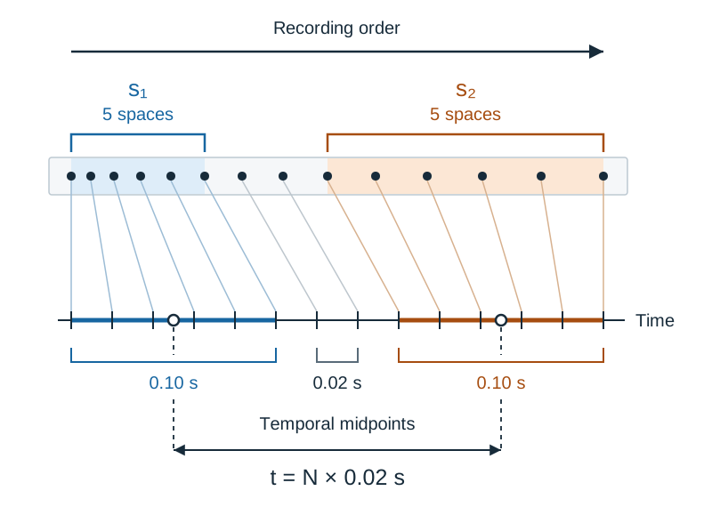
• The time interval between two consecutive dots (one space) is $\Delta t = \frac{1}{50}\text{ s} = 0.02\text{ s}$.
• As a trolley attached to the tape accelerates, the distance between successive dots increases steadily.
• Initial velocity ($u$): Measure the length $s_1$ of an early run of 5 spaces ($t_1 = 5 \times 0.02 = 0.10\text{ s}$), giving $u = \frac{s_1}{0.10}$.
• Final velocity ($v$): Measure the length $s_2$ of a later run of 5 spaces ($t_2 = 5 \times 0.02 = 0.10\text{ s}$), giving $v = \frac{s_2}{0.10}$.
• Time interval ($t$): Count the number of spaces $N$ between the midpoints of the two chosen 5-space sections. The elapsed time is $t = N \times 0.02\text{ s}$.
• Calculate acceleration from $a = \frac{v - u}{t}$.

Light Gates and Linear Air Track

An air track pumps air through tiny holes in a track to float a metal rider on an air cushion, virtually removing friction.

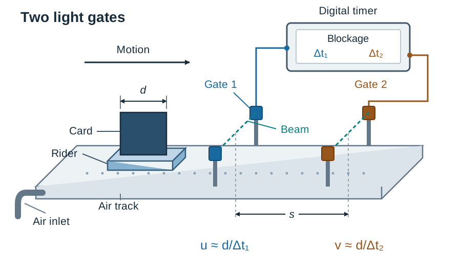
• Setup: Mount an interrupt card of measured width $d$ (e.g. $0.050\text{ m}$) on the rider. Position two photogates connected to a digital timer along the track, separated by distance $s$ (e.g. $0.60\text{ m}$).
• Measurements: The timer records how long the card blocks each light beam: $\Delta t_1$ at Gate 1 and $\Delta t_2$ at Gate 2. Because $d$ is small, $\frac{d}{\Delta t}$ gives the average velocity while passing each gate, which closely approximates the instantaneous velocity at the gate.
• Velocities: $u = \frac{d}{\Delta t_1}$ and $v = \frac{d}{\Delta t_2}$.
• Calculation: Compute acceleration using $a = \frac{v^2 - u^2}{2s}$. For instance, if $\Delta t_1 = 0.100\text{ s}$ and $\Delta t_2 = 0.050\text{ s}$, then $u = \frac{0.050}{0.100} = 0.50\text{ m s}^{-1}$ and $v = \frac{0.050}{0.050} = 1.0\text{ m s}^{-1}$. With $s = 0.60\text{ m}$, $a = \frac{(1.0)^2 - (0.50)^2}{2(0.60)} = \frac{0.75}{1.20} = 0.63\text{ m s}^{-2}$.

Measuring g by Free Fall and Pendulum (Primary Data)

You must be able to verify at least one model for $g$ with your own measurements and all four models using secondary data supplied to you. Free fall and the simple pendulum are standard laboratory methods.

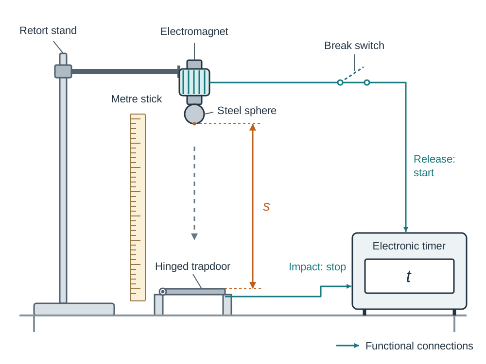
Method 1: Free-Fall Apparatus

Diagram Description

Draw a vertical retort stand with an electromagnet clamped at the top holding a small steel sphere. Directly beneath the sphere, draw a horizontal hinged trapdoor (impact pad) mounted on a bench. Connect the electromagnet and the trapdoor to an electronic digital timer, with a break switch in the electromagnet circuit. Draw a vertical double-headed arrow labelled distance $s$ from the bottom of the ball to top of the trapdoor, and place a vertical metre stick alongside.

What You Measure

• Distance $s$ from the bottom of the suspended sphere to the top of the trapdoor using the metre stick.
• Time of fall $t$ recorded by the millisecond timer when the switch releases the ball and the ball strikes the trapdoor.

Graph and Slope Determination

Starting from rest ($u = 0$), $s = \frac{1}{2}gt^2$. Plot $s$ against $t^2$ on graph paper, placing $s$ on the vertical axis and $t^2$ on the horizontal axis. Draw a straight line of best fit through the origin. Since $y = mx$ matches $s = (\frac{1}{2}g)t^2$, the slope is $m = \frac{1}{2}g$, which gives:

$$g = 2 \times \text{slope}$$

Using several drop heights and plotting a graph averages out random timing variations and confirms that $s \propto t^2$.

Precautions and Error Sources

• Measure distance $s$ strictly from the bottom of the ball to top of the trapdoor, because the bottom surface breaks the contact on impact.
• Reduce residual magnetism in the core of the electromagnet, which delays release and makes measured times too long (producing an underestimated $g$). Minimise this by using the lowest holding current possible or sticking a small piece of paper to the magnet pole.
• Use a dense, small steel ball to make air resistance negligible.

Method 2: Simple Pendulum

Diagram Description

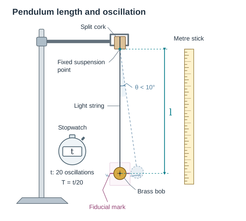
Draw a retort stand clamping a split cork. Between the two halves of the cork, show a light string gripping firmly and hanging vertically, attached to a small, dense brass pendulum bob. Label the lower edge of the cork "fixed point of suspension". Draw a vertical arrow labelled length $l$ from the bottom of the split cork to the centre of the bob. Place a metre stick beside the arrangement and show a stopwatch.

What You Measure

• Length $l$ from the bottom of the split cork to the centre of the bob (using a metre stick to the top of the bob, plus callipers to measure bob radius).
• Time $t$ for 20 complete oscillations using a stopwatch, then calculate periodic time $T = \frac{t}{20}$.

Graph and Slope Determination

For small oscillations, $T = 2\pi\sqrt{\frac{l}{g}}$. Squaring gives $T^2 = \frac{4\pi^2}{g}l$, which rearranges to $l = \left(\frac{g}{4\pi^2}\right)T^2$. Plot length $l$ on the vertical axis against $T^2$ on the horizontal axis. Draw a straight line of best fit through the origin. The slope is $m = \frac{g}{4\pi^2}$, which gives:

Precautions and Error Sources

• Keep the angle of swing small (less than about $10^\circ$) so that the simple harmonic motion approximation holds.
• Clamp the string firmly in a split cork to ensure a fixed, unchanging pivot point.
• Measure length $l$ to the centre of the bob, not just to the hook or top edge.
• Time at least 20 complete oscillations and divide to find $T$, which drastically cuts the percentage impact of human reaction time.
• Count oscillations using a fiducial mark placed behind the equilibrium position, timing as the bob swings past its fastest point in the centre.
• Ensure the bob oscillates strictly in a single vertical plane without wobbling in a conical path.

Four Mathematical Models for g

There are four different ways to model $g$. You should be able to test at least one with your own measurements, and all four using data you are given.

1. Free Fall from Rest: $g = \frac{2s}{t^2}$

Originating from the kinematic equation $s = ut + \frac{1}{2}at^2$ with $u = 0$ and $a = g$. Verified by dropping objects over measured heights and plotting $s$ against $t^2$.

2. Simple Pendulum: $g = \frac{4\pi^2 l}{T^2}$

Derived from the restoring force on a suspended mass undergoing small-angle angular displacement. Verified by measuring the period of swing across various pendulum lengths and plotting $l$ against $T^2$.

3. Universal Gravitation: $g = \frac{GM}{r^2}$

Derived by equating the gravitational attraction on an object of mass $m$ to its weight: $mg = \frac{GMm}{r^2}$, where $G = 6.674 \times 10^{-11}\text{ N m}^2\text{ kg}^{-2}$, $M$ is the mass of the planetary body, and $r$ is the distance from its centre. This model explains why $g$ decreases as altitude increases and why $g$ varies on other celestial bodies.

4. Fluid Column Pressure: $g = \frac{P}{h\rho}$

Derived from fluid statics, where $P$ is the pressure due to the liquid alone at depth $h$ (total pressure minus atmospheric pressure) and $\rho$ is fluid density ($P = h\rho g$). Rearranging gives $g = \frac{P}{h\rho}$.

Key terms

Acceleration

The rate of change of velocity with respect to time.

Velocity

The rate of change of displacement with respect to time.

Displacement

Distance in a given direction.

Distance

The total length of the path travelled by an object; a scalar quantity.

Speed

The rate of change of distance with respect to time.

Uniform acceleration

Constant acceleration; motion in which velocity changes by equal amounts in equal intervals of time.

Instantaneous acceleration

The acceleration of an object at a specific instant in time, found from the slope of the tangent to a velocity-time graph.

Deceleration

A decrease in speed, occurring whenever the acceleration vector opposes the velocity vector.

Acceleration due to gravity (g)

The acceleration produced by the gravitational attraction of a celestial body on an object in free fall near its surface.

Vector

A physical quantity that has both magnitude and direction.

Scalar

A physical quantity that has magnitude only, with no direction.