Statistics Inferential Statistics

Sampling and the Central Limit Theorem

A population includes every single individual or item you want to study, whereas a sample is just a subgroup picked from that population. Any numerical measurement describing the population is a parameter, like the population mean $\mu$ or population proportion $p$. A measurement calculated from your sample is a statistic, such as the sample mean $\bar{x}$ or sample proportion $\hat{p}$. Parameters stay fixed, but statistics change from sample to sample. This natural bounce between different samples is called sampling variability.

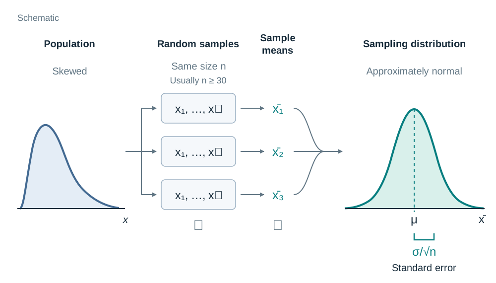
If you took hundreds of random samples of size $n$ from the same population and calculated $\bar{x}$ for each one, the spread of those sample means forms the sampling distribution of the mean. The Central Limit Theorem tells us that whenever the sample size is large enough (usually $n \geq 30$), this sampling distribution is approximately normal, even if the parent population is skewed or irregular. The mean of this sampling distribution equals the true population mean $\mu$, and its standard deviation is known as the standard error, given by $\sigma_{\bar{x}} = \frac{\sigma}{\sqrt{n}}$. In exam questions where the population standard deviation $\sigma$ is unknown, you can safely use the sample standard deviation $s$ as an approximation when $n \geq 30$.

Confidence Intervals for Means and Proportions

A single sample statistic gives you a point estimate, but it tells you nothing about how close you are to the true figure. A confidence interval fixes this by giving a plausible band of values backed by a chosen confidence level. At Higher Level, you will nearly always calculate 95% confidence intervals, which use the critical value $z = 1.96$ from the standard normal tables.

For a population mean, calculate the 95% interval using $\left[\bar{x} - 1.96\frac{s}{\sqrt{n}}, \bar{x} + 1.96\frac{s}{\sqrt{n}}\right]$. For example, if a sample of $100$ students has a mean study time of $20$ hours with standard deviation $4$ hours, the standard error is $\frac{4}{\sqrt{100}} = 0.4$. The margin of error is $1.96 \times 0.4 = 0.784$, giving an interval from $19.216$ to $20.784$ hours.

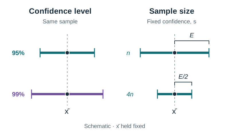
For a population proportion, the 95% interval is $\hat{p} \pm 1.96\sqrt{\frac{\hat{p}(1-\hat{p})}{n}}$, where $\hat{p} = \frac{x}{n}$ is the sample proportion. The margin of error is largest when $\hat{p} = 0.5$, because $\hat{p}(1 - \hat{p})$ cannot exceed $0.25$. This gives the maximum 95% margin of error $E = 1.96\sqrt{\frac{0.25}{n}} = \frac{0.98}{\sqrt{n}} \approx \frac{1}{\sqrt{n}}$. For example, with a sample of $n = 900$, the maximum margin of error is $E \approx \frac{1}{\sqrt{900}} = \frac{1}{30} \approx 0.033$ (or $3.3\%$). To find the sample size required for a desired margin of error $E$, rearrange to $n \approx \frac{1}{E^2}$; for example, achieving a margin of $\pm 4\%$ ($E = 0.04$) requires $n = \frac{1}{0.04^2} = 625$. You should note how confidence levels and sample sizes behave. If you want a higher level of certainty, like 99% ($z = 2.575$), your margin of error grows and your interval gets wider. Conversely, because $n$ sits under a square root in the denominator, you have to quadruple your sample size if you want to cut the margin of error in half.

Hypothesis Testing and P-Values

A hypothesis test is a formal method to decide whether sample evidence contradicts an existing claim. You start by stating two competing claims: the null hypothesis ($H_0$), which represents no change or the status quo, and the alternative hypothesis ($H_1$), which claims a genuine difference. At Higher Level, tests on a population mean are two-tailed, so you write $H_0: \mu = k$ and $H_1: \mu \neq k$.

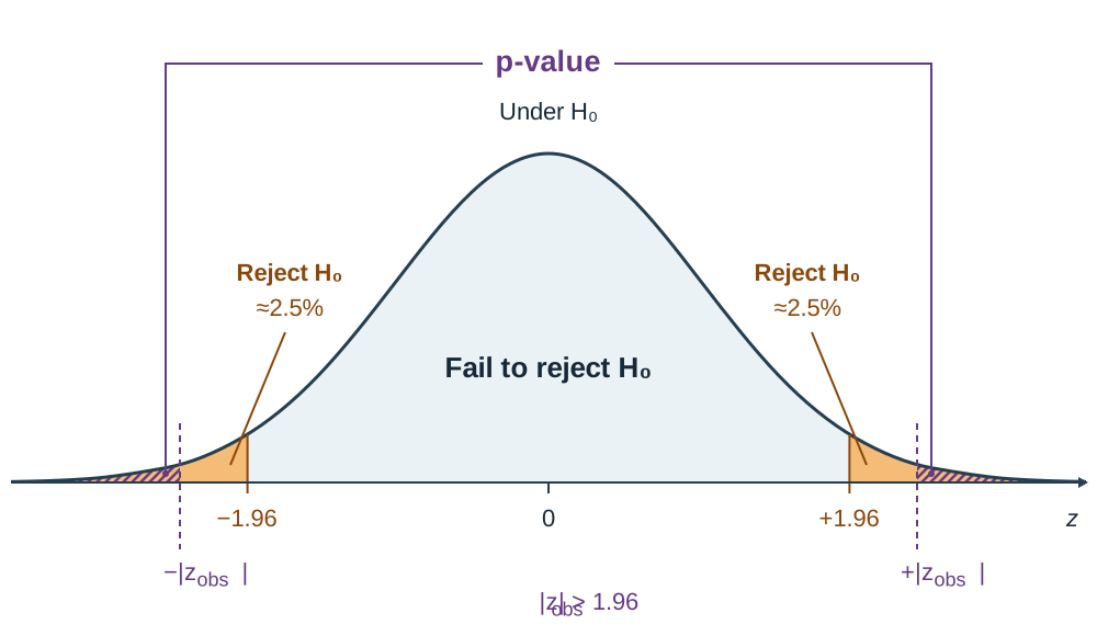
To test the claim, convert your sample mean into a test statistic using $z = \frac{\bar{x} - \mu}{\frac{s}{\sqrt{n}}}$. At the standard 5% significance level, the critical values are $\pm 1.96$. If your test statistic lands in the critical region ($z \geq 1.96$ or $z \leq -1.96$, meaning $|z| \geq 1.96$), you reject $H_0$. If $|z| < 1.96$, you fail to reject $H_0$.

You can also make decisions using a p-value, which measures the exact probability of getting a result at least as extreme as your sample if $H_0$ were true. For a two-tailed test, look up your positive z-score in the log tables, find the tail area $1 - P(Z \leq |z|)$, and double it: $p = 2(1 - P(Z \leq |z|))$. If $p < 0.05$, reject $H_0$; if $p \geq 0.05$, fail to reject $H_0$. Always wrap up with a sentence in plain English stating what your decision means in the context of the question.

Testing hypotheses about a population proportion

To test a claim about a population proportion at the 5% level of significance using the margin of error:

1. State the null and alternative hypotheses: $H_0: p = k$ and $H_1: p \neq k$.
2. Calculate the sample proportion $\hat{p} = \frac{x}{n}$ and the margin of error $E$ (using $1.96\sqrt{\frac{\hat{p}(1-\hat{p})}{n}}$ or the maximum margin $\frac{1}{\sqrt{n}}$).
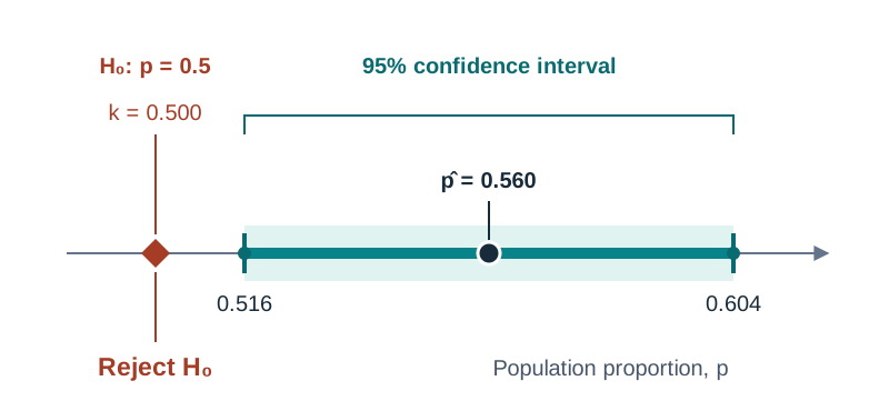
3. Set up the 95% confidence interval: $[\hat{p} - E, \hat{p} + E]$.
4. Make your decision: reject $H_0$ if $k$ lies outside the confidence interval; fail to reject $H_0$ if $k$ lies inside the interval.
5. State your conclusion in the context of the problem.

For example, test the claim that support for the transport initiative is 50% ($H_0: p = 0.5$ versus $H_1: p \neq 0.5$) using the survey in Worked Example 2 below, where $280$ of $500$ voters supported it ($\hat{p} = 0.56$):

• The 95% confidence interval is $[0.516, 0.604]$ (or $[0.515, 0.605]$ using the maximum margin $\frac{1}{\sqrt{500}} \approx 0.045$).
• Because $0.5$ lies outside this interval, we reject $H_0$.
• There is sufficient evidence at the 5% level of significance that public support is not 50%.

Key terms

Population

The entire collection of individuals, items, or scores that you want to draw conclusions about.

Sample

A subset selected from a population to represent the whole group in an investigation.

Parameter

A fixed numerical characteristic describing an entire population, such as the mean $\mu$ or proportion $p$.

Statistic

A numerical value calculated from sample data, like $\bar{x}$ or $\hat{p}$, which varies from sample to sample.

Sampling Variability

The natural variation in sample statistics that occurs when different random samples are drawn from the same population.

Central Limit Theorem

A theorem stating that the sampling distribution of the mean approaches a normal distribution as sample size grows ($n \geq 30$), regardless of the population shape.

Standard Error

The standard deviation of a sampling distribution, representing the typical distance between a sample statistic and the true population parameter.

Null Hypothesis ($H_0$)

The baseline statement assuming no difference, no change, or that an established claim is true, written with an equals sign.

Alternative Hypothesis ($H_1$)

The statement you adopt if the sample provides convincing evidence against the null hypothesis, written as not equal to ($\neq$) for two-tailed tests.

P-value

The probability of getting a sample statistic as extreme as, or more extreme than, the observed value, assuming the null hypothesis is true.

Critical Region

The set of extreme test statistic values (such as $|z| \geq 1.96$ at the 5% level) that leads you to reject the null hypothesis.