Probability Foundations

Counting Principles

The Fundamental Principle of Counting tells us that if one action can happen in $m$ ways and a second action can happen in $n$ ways, both together can happen in $m \times n$ ways. When you face an arrangement problem with conditions, draw out empty boxes for each spot and fill in the restricted spots first.

When ordering $n$ distinct items in a line, the total number of arrangements is $n! = n \times (n-1) \times \dots \times 2 \times 1$, with $0!$ defined as $1$. If order matters, such as assigning places or creating access codes, you are dealing with a permutation, written as $^n P_r = \frac{n!}{(n-r)!}$. When order does not matter, like picking a team or a committee, you use a combination, written as $\binom{n}{r}$ or $^n C_r = \frac{n!}{r!(n-r)!}$. A handy symmetry to remember is the Twin Rule, $\binom{n}{r} = \binom{n}{n-r}$.

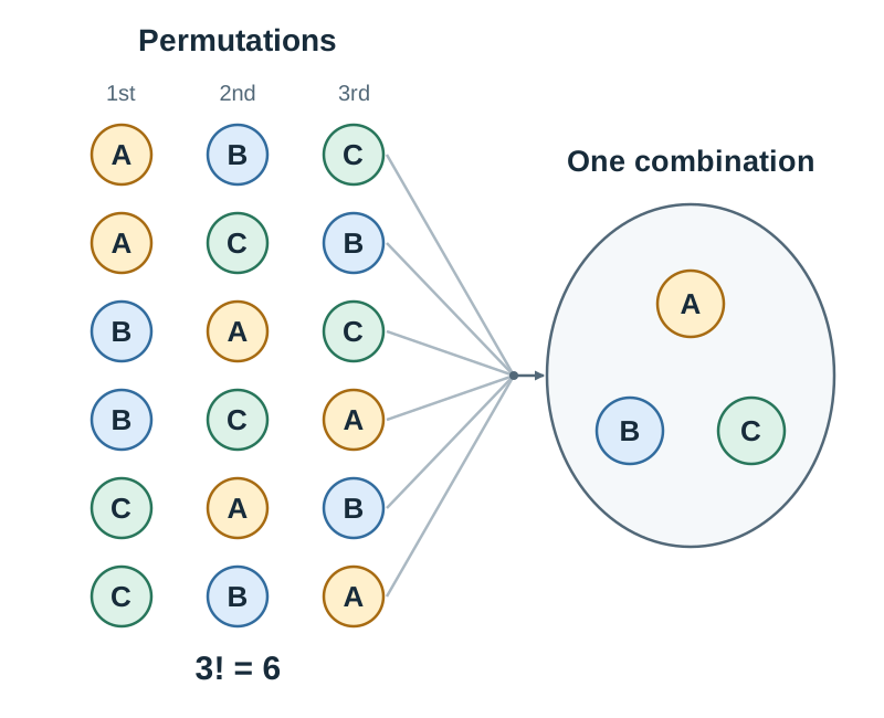
For example, to choose a committee of 4 from 6 girls and 4 boys with exactly 2 girls and 2 boys, by the Fundamental Principle of Counting, each choice of 2 girls can go with each choice of 2 boys: $\binom{6}{2} \times \binom{4}{2} = 15 \times 6 = 90$ ways. To find the probability that a randomly chosen 4-person committee has exactly 2 girls and 2 boys, divide this count by the total possible committees: $\frac{90}{\binom{10}{4}} = \frac{90}{210} = \frac{3}{7}$.

If people or objects must sit or stand together, glue them together into a single unit, count the arrangements of the new units, and then multiply by the internal arrangements within the grouped unit.

Basic Probability Rules and Venn Diagrams

Every probability sits between $0$ (an impossible event) and $1$ (a certain event). When every single outcome is equally likely, the probability of an event $E$ is simply $P(E) = \frac{\#E}{\#S}$, which is the count of favourable outcomes divided by the total number of outcomes in the sample space $S$.

In probability, set notation provides precision: $A \cup B$ means $A$ or $B$ (or both), $A \cap B$ means $A$ and $B$, and $E'$ means $E$ does not happen (the complement: $P(E') = 1 - P(E)$). Venn diagrams display overlapping events clearly. For example, in a group of 30 students, 18 play football, 12 play hurling, and 5 play both. Always fill in the intersection first: 5 play both, so $18 - 5 = 13$ play football only, $12 - 5 = 7$ play hurling only, and $30 - (13 + 5 + 7) = 5$ play neither. From the diagram, $P(\text{at least one sport}) = \frac{13 + 5 + 7}{30} = \frac{25}{30} = \frac{5}{6}$. For two-stage experiments such as rolling two dice, a two-way grid systematically lists all $6 \times 6 = 36$ equally likely outcomes.

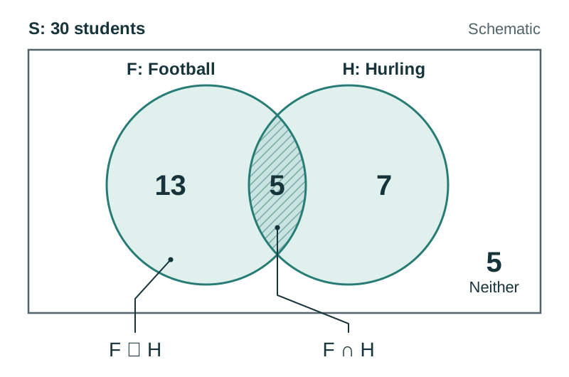
For any two events $A$ and $B$, the general addition rule states that $P(A \cup B) = P(A) + P(B) - P(A \cap B)$. We subtract the intersection $P(A \cap B)$ so that outcomes belonging to both sets are not counted twice. If two events are mutually exclusive, they cannot happen at the same time, meaning $A \cap B = \varnothing$ and $P(A \cap B) = 0$. In that case, the rule simplifies to $P(A \cup B) = P(A) + P(B)$.

Independence and Tree Diagrams

Two events $A$ and $B$ are independent when the occurrence of one has no influence on the chance of the other occurring. The formal test for independence is $P(A \cap B) = P(A) \times P(B)$. When an exam question asks you to investigate whether two events are independent, never just assume they are; compute the product $P(A) \times P(B)$, find $P(A \cap B)$ separately, and state clearly whether they match.

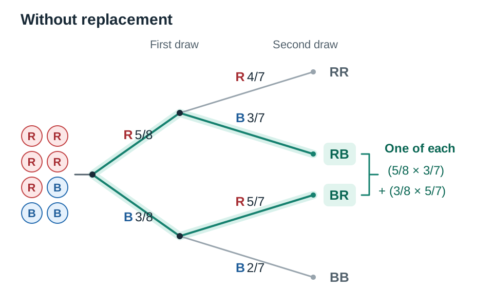
Tree diagrams give you a reliable visual map for multistage experiments. You multiply probabilities along consecutive branches to find the probability of a path, and you add the probabilities of separate valid paths. With sampling without replacement, the total on the second branch drops by 1. The count for a type drops by 1 only if that type was taken on the first pick. For example, after a red is removed from 5 red and 3 blue: $P(\text{red}) = \frac{4}{7}$ and $P(\text{blue}) = \frac{3}{7}$. Always check that the branches sprouting from any single node add up to $1$.

Conditional Probability

We write $P(A|B)$ for the probability of $A$ when we know that $B$ has happened (or is true). $B$ does not have to happen first. For example, $P(\text{condition} \mid \text{positive test})$ evaluates the chance that a person has a medical condition given that their test result was positive. The standard definition is $P(A|B) = \frac{P(A \cap B)}{P(B)}$, or in counting terms, $\frac{\#(A \cap B)}{\#B}$.

The condition $B$ becomes your new, restricted sample space, which is why $P(B)$ sits in the denominator. For example, in a class of 15 boys (5 wearing glasses) and 10 girls (3 wearing glasses), there are 8 students wearing glasses in total. If a student who wears glasses is selected, the probability they are female is $P(\text{Female} \mid \text{Glasses}) = \frac{\#(\text{Female} \cap \text{Glasses})}{\#\text{Glasses}} = \frac{3}{8}$.

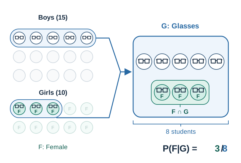
Conditional statements do not commute: $P(A|B) \neq P(B|A)$ in general. For medical screening questions and other reverse-probability problems, sketch a tree diagram or a contingency grid. First work out the overall probability of the observed outcome by adding the relevant branch paths, then divide the target branch by that total.

At Least One and Expected Value

Phrases like 'at least once' are an immediate signal to consider the complement rule. Instead of adding up cases for one, two, three, or more successes, use $P(\text{at least one}) = 1 - P(\text{none})$. If each trial fails with probability $q$, then $P(\text{none in } n \text{ trials}) = q^n$, so form the inequality $1 - q^n > k$. Rearrange to isolate the power ($q^n < 1 - k$), take natural logarithms on both sides ($n \ln(q) < \ln(1 - k)$), and reverse the inequality sign when dividing by $\ln(q)$, since the logarithm of a probability between $0$ and $1$ is negative.

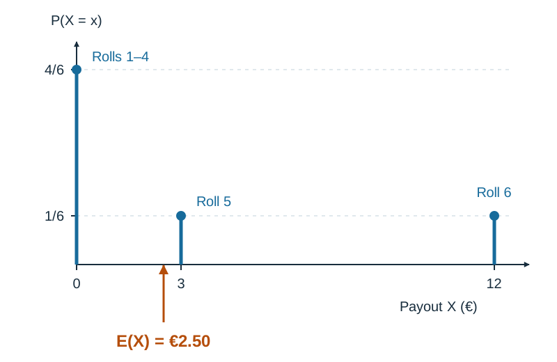
The expected value $E(X) = \sum x \cdot P(x)$ tells you the long-run average outcome per play if an experiment were repeated many times. $E(X)$ is a long-run average, so it need not be one of the possible outcomes. In a fair game, the expected net gain is zero, meaning the expected payout matches the cost to enter. For practical decision-making problems, calculate the expected cost or return for each option and select the one that makes the best financial sense.

Key terms

Sample space

The complete set of all possible outcomes of a probability experiment, denoted by S.

n!

The factorial of n, giving the number of ways to arrange n distinct items in order: n × (n - 1) × ... × 1.

Combination

A selection of items from a larger collection where the order of choosing does not matter, calculated as nCr.

Permutation

An arrangement of r items chosen from n distinct items where the order of selection matters, calculated as nPr.

Independent

Two events are independent if the occurrence of one does not alter the probability of the other, satisfying P(A ∩ B) = P(A) × P(B).

Mutually exclusive

Events that cannot happen simultaneously, meaning their intersection is empty and P(A ∩ B) = 0.

Conditional probability

The probability of an event A occurring given that event B has occurred or is true, calculated as P(A|B) = P(A ∩ B) / P(B).

Expected value

The weighted average of all possible numerical outcomes of a random variable, given by E(X) = Σ x · P(x).

Fair game

A game in which the expected winnings equal the entry fee, so the expected net return is zero.