Probability Distributions Notes | Leaving Cert Mathematics

Probability distributions provide the mathematical models for handling uncertainty and variability. We use discrete models like the Binomial Distribution for counting successes in repeated trials and continuous models like the Normal Distribution for real-world measurements. These tools, alongside expected value calculations, allow you to analyse data and make informed decisions in both theoretical and practical contexts.

Expected Value and Decision-Making

Expected value, E(X), is the average outcome of a random process over the long term. Calculate it by summing the products of each outcome (x) and its probability (P(x)): E(X) = Σ x · P(x). A game is a fair game if the expected net gain is €0, meaning the expected prize equals the cost to play. If the expected net gain is positive, you gain on average; if negative, you have an 'expected loss'. When setting a premium or comparing decisions, calculate the expected cost or return for each option to determine the best choice.

Binomial Distribution and Bernoulli Trials

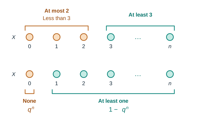
The binomial distribution models the number of successes (r) in n independent Bernoulli trials. A trial has two outcomes: success (p) or failure (q = 1 − p). The probability of exactly r successes is P(X = r) = nCr · p^r · q^(n-r). Answer binomial questions with this formula, adding terms where needed. You are not required to approximate a binomial with the normal curve. Check four conditions before use: n is fixed; binary outcomes; trials are independent; and p is constant. If picking without replacement, probabilities change, so trials are not independent and you must use combinations or tree diagrams instead. Common wording translates to maths as: 'at most 2' = P(0)+P(1)+P(2); 'less than 3' = P(0)+P(1)+P(2); 'at least 3' = 1 − [P(0)+P(1)+P(2)]; and at least one = 1 − P(none), which is 1 − q^n.

Integer outcomes from 0 to n, grouped into 0–2 and 3–n, with a second grouping separating none from at least one.

Independence, Conditional Probability, and Sequences

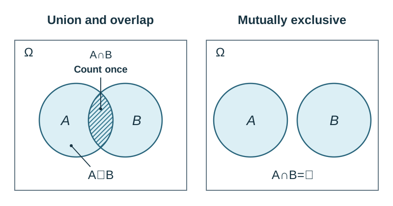
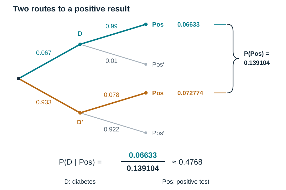
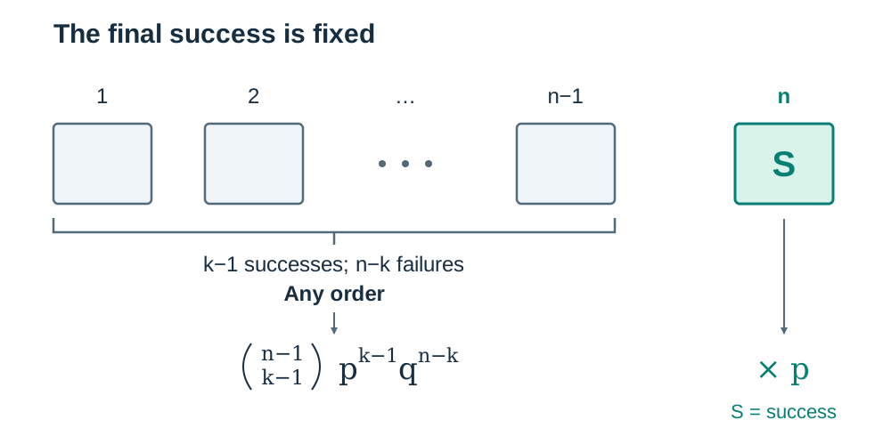
Two events are independent if the occurrence of one does not change the probability of the other; test this using P(A ∩ B) = P(A) × P(B). Addition rule: P(A ∪ B) = P(A) + P(B) − P(A ∩ B). We subtract the overlap so it is not counted twice. If A and B are mutually exclusive, P(A ∩ B) = 0, so P(A ∪ B) = P(A) + P(B). Use tree diagrams for sequential events; multiply along branches to find the path probability and add paths for 'OR' conditions. For conditional probability P(A | B), use the formula P(A | B) = P(A ∩ B) / P(B). The denominator is always the event after 'given'. Along a tree, P(A ∩ B) = P(A) × P(B | A). In general P(A | B) ≠ P(B | A). For example, if 6.7% of people have diabetes (D) and a test gives a positive result (Pos) for 99% of people with diabetes but 7.8% of people without: P(D ∩ Pos) = 0.067 × 0.99 = 0.06633, and P(D′ ∩ Pos) = 0.933 × 0.078 = 0.072774. Total P(Pos) = 0.06633 + 0.072774 = 0.139104 ≈ 0.1391. Then P(D | Pos) = 0.06633 / 0.139104 ≈ 0.4768. In context, fewer than half of those who test positive actually have diabetes, even though P(Pos | D) = 0.99. For the kth success on the nth trial, the first (n − 1) trials must have (k − 1) successes, then trial n must be a success: P = [ⁿ⁻¹C_{k−1} · p^{k-1} · q^{n-k}] · p.

Overlapping events A and B have their union shaded and intersection hatched; a second sample space shows disjoint events.

A probability tree highlights positive results with and without diabetes, whose probabilities sum to 0.139104.

Trials 1 through n−1 contain k−1 successes in any order; trial n is a compulsory success.

Normal Distribution

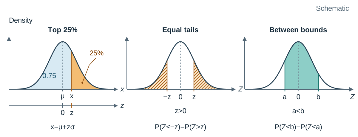
The normal curve is symmetric and bell-shaped. We convert values to a z-score to use the tables: z = (x − μ) / σ, where μ is the mean and σ is the standard deviation. A z-score tells you how many standard deviations a value is from the mean. The Formulae and Tables booklet gives P(Z ≤ z) for positive z. Use: P(Z > z) = 1 − P(Z ≤ z); P(Z ≤ −z) = 1 − P(Z ≤ z); and P(a ≤ Z ≤ b) = P(Z ≤ b) − P(Z ≤ a). For 'top 25%' questions, look up 0.75 in the body of the tables to find z, then solve x = μ + zσ.

Three schematic normal curves show a top-quarter cutoff, equal opposite tails, and an interval between two bounds.

Key terms

Bernoulli trial: An experiment with exactly two outcomes: success (p) or failure (q).
binomial distribution: The distribution of the number of successes in n independent trials.
independent: Events where the occurrence of one does not affect the other: P(A ∩ B) = P(A) × P(B).
mutually exclusive: Events that cannot occur at the same time: P(A ∩ B) = 0.
conditional probability: The probability of A given B has occurred: P(A | B) = P(A ∩ B) / P(B). In general, P(A | B) ≠ P(B | A).
expected value: The long-term average outcome: E(X) = Σ x · P(x).
fair game: A game where the expected net gain is zero.
z-score: A measure of how many standard deviations a data point is from the mean: z = (x − μ) / σ.

Check yourself

If P(A)=0.4, P(B)=0.5, and P(A∩B)=0.2, are A and B independent?
Yes. 0.4 × 0.5 = 0.2, which equals P(A∩B).
A game costs €5 to play and is fair. What is the expected value of the prize?
€5. The expected net gain is 0, so the expected prize equals the cost.
In a normal distribution with mean 50 and standard deviation 8, find P(X < 42).
z = (42-50)/8 = -1. P(Z < -1) = 1 - P(Z < 1) = 1 - 0.8413 = 0.1587.

Probability Distributions