Functions

Essential Vocabulary

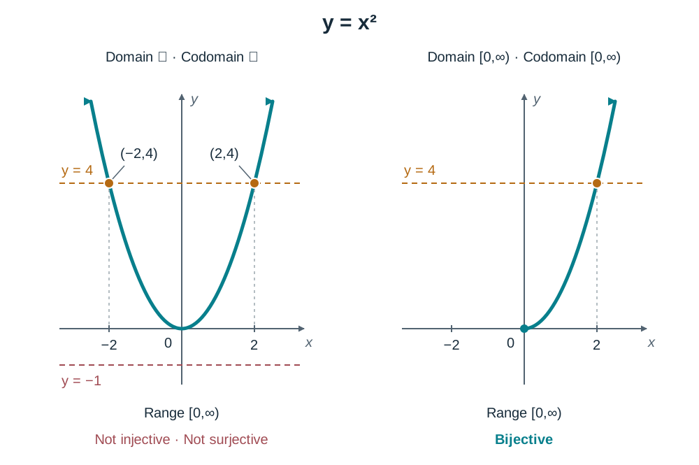
We write a function as $f: A \to B$, where set $A$ is the domain and set $B$ is the codomain. The domain contains every allowed input value. The codomain is the set of possible target values, but the range is the actual collection of outputs your function delivers. A function is injective (or one-to-one) if distinct inputs always produce distinct outputs; on a sketch, any horizontal line hits an injective curve at most once. A function is surjective (or onto) if the range matches the codomain completely, meaning every target value gets hit at least once. When a function is both injective and surjective, we call it bijective. Only bijective functions have true inverses, because each output must trace back to one distinct starting input. For example, consider $f: \mathbb{R} \to \mathbb{R}$ where $f(x) = x^2$. It is not injective because $f(2) = f(-2) = 4$, so the horizontal line $y = 4$ meets the graph twice. It is also not surjective because no real number $x$ produces $x^2 = -1$. However, if we restrict the domain and codomain to $f: [0, \infty) \to [0, \infty)$, the function becomes bijective and has an inverse, $f^{-1}(x) = \sqrt{x}$.

Quadratic Functions

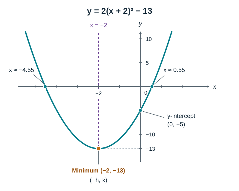
Standard quadratics take the form $f(x) = ax^2 + bx + c$. When $a > 0$, the curve opens upward into a U-shape; when $a < 0$, it opens downward. While you can find turning points using calculus, the syllabus specifically expects you to write quadratics in completed square form: $f(x) = a(x + h)^2 + k$. To do this, factor $a$ out of the $x^2$ and $x$ terms first, halve the new $x$-coefficient, square that value, and balance it inside the brackets. From $a(x + h)^2 + k$, the vertex sits at $(-h, k)$ and the axis of symmetry is the vertical line $x = -h$. If $a > 0$, the turning point is a minimum; if $a < 0$, it is a maximum. Solving $a(x + h)^2 + k = 0$ gives you the roots directly without needing the $-b$ formula. To sketch, plot the turning point $(-h, k)$, the roots (if any), and the $y$-intercept $f(0)$, then draw a U-shape if $a > 0$ or an ∩-shape if $a < 0$, symmetric about $x = -h$.

Cubic Functions

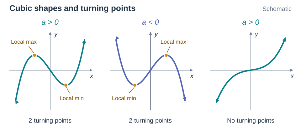
A cubic function has the form $f(x) = ax^3 + bx^2 + cx + d$ with $a \neq 0$. If $a > 0$, the curve starts low on the left and rises to the top right; if $a < 0$, it starts high on the left and finishes low. Because cubic graphs stretch from negative infinity to positive infinity, every cubic must cross the $x$-axis at least once, giving between one and three real roots. They can have up to two turning points—one local maximum and one local minimum—though some cubics increase or decrease throughout their entire domain with no turning points at all. In exam questions, you often read approximate roots and turning points straight from a supplied plot, or use the factor theorem to break the cubic into a linear and a quadratic factor.

Exponential and Logarithmic Functions

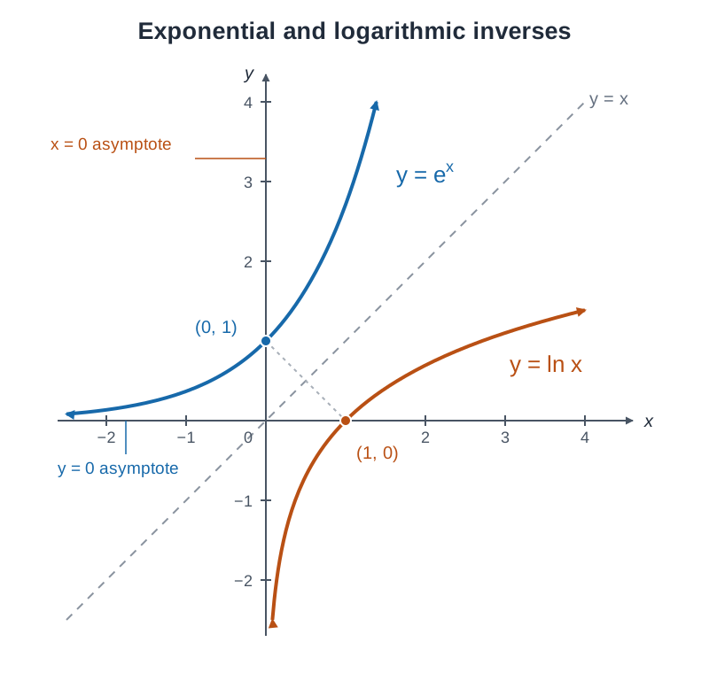
An exponential function $f(x) = ab^x$ places the variable right in the power. For $b > 1$ (with $a > 0$), the function models growth, passing through $(0, a)$ and rising steeply. When $0 < b < 1$ (with $a > 0$), the graph falls instead (decay); it still passes through $(0, a)$. The special base $e \approx 2.718$ is used in growth and decay models. Its inverse is $\ln x$, which means $\log_e x$, so $\ln(e^x) = x$ and $e^{\ln x} = x$ for $x > 0$. Also, $e^x > 0$ for every real $x$. The $x$-axis acts as a horizontal asymptote: the curve approaches $y = 0$ as $x$ becomes very negative (for growth), but it never touches or crosses zero. The logarithmic function $g(x) = \log_b x$ is the inverse of $y = b^x$, so reflecting the graph of $y = b^x$ in the line $y = x$ gives the graph of $y = \log_b x$. A log graph only accepts positive inputs ($x > 0$), has a vertical asymptote along the $y$-axis ($x = 0$), and always cuts through $(1, 0)$ because $\log_b 1 = 0$ for any valid base.

Inverse Functions and Graphical Solutions

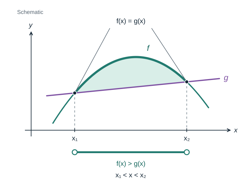
An inverse function $f^{-1}(x)$ undoes whatever operation $f(x)$ performed. To work out an inverse formula algebraically, write $y = f(x)$, rearrange the terms to isolate $x$ completely on one side, and then swap your variables so the rule is written in terms of $x$. On a graph, $f$ and $f^{-1}$ are mirror reflections of each other across the line $y = x$. If a point $(p, q)$ sits on the graph of $f$, the swapped point $(q, p)$ must lie on the graph of $f^{-1}$. The solutions of $f(x) = 0$ are the $x$-values where the graph crosses the $x$-axis, and the solutions of $f(x) = k$ are the $x$-values where the graph meets the horizontal line $y = k$. Graph readings are approximate. When an exam asks you to solve $f(x) = g(x)$ graphically, find the $x$-coordinates where the two plots intersect. If an inequality asks for $f(x) > g(x)$, identify the $x$-intervals where the curve of $f$ sits vertically higher than $g$.

Trigonometric Graphs

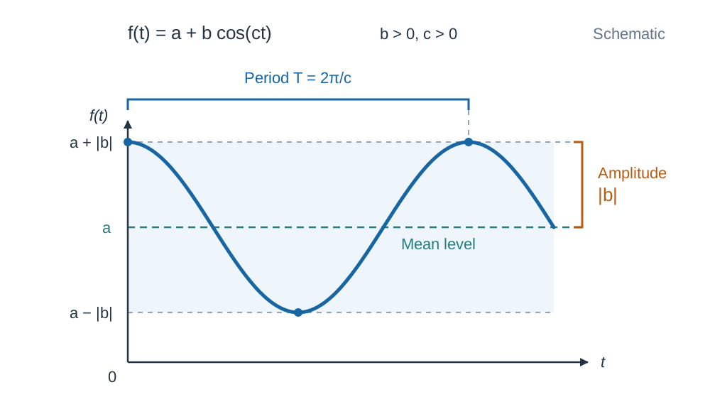
Leaving Cert models for tides, temperatures, and alternating currents often rely on waves of the form $f(t) = a + b\sin(ct)$ or $f(t) = a + b\cos(ct)$. Here, $a$ represents the mean level or vertical shift, which sits midway between the maximum and minimum values: $a = \frac{\text{Max} + \text{Min}}{2}$. The number $|b|$ gives the amplitude, calculated as $\frac{\text{Max} - \text{Min}}{2}$. The range runs from $a - |b|$ up to $a + |b|$. The period is the time or horizontal distance needed to complete one full cycle. In radians, you calculate the period using $T = \frac{2\pi}{c}$, which lets you find $c$ whenever the peak-to-peak time is known.

Key terms

Domain

The complete set of all allowable input values ($x$-values) for which a function is defined.

Bijective

A function that is simultaneously injective (one-to-one) and surjective (onto), meaning every element in the codomain connects to exactly one input.

Turning Point

A point on a curve where the gradient changes sign, forming a local maximum or local minimum.

Asymptote

A straight line that a curve gets closer and closer to as $x$ or $y$ becomes very large (or very negative). For example, $y = e^x$ approaches $y = 0$ as $x \to -\infty$.

Inverse Function

A function, written $f^{-1}$, that reverses the transformation of $f$ so that $f^{-1}(f(x)) = x$ and $f(f^{-1}(x)) = x$.

Period

The horizontal length along the domain over which a repeating function completes one full cycle.