

Some problems are too complicated, too dangerous or too slow to study for real: you cannot crash a hundred cars to test a bumper, and there is no single formula that tells you how long the canteen queue will be at 1 p.m. Instead, we build a simplified version of the system on a computer — a model — and run it forward in time to see what happens. That is simulation. This note covers what a model is, how abstraction decides what goes into it, how to test different scenarios and compare the results, how simulations built from many independent 'agents' produce surprising group behaviour, and how heuristics give good-enough answers when an exact one would take too long.
Models, Abstraction, and Abstract Models
A model is a simplified representation of a real-world object, system, or process. Every model is built for a clear purpose. For instance, a traffic model might investigate how changing traffic light timings alters queue lengths at a busy crossroads. To answer that question, the model captures essential variables such as arrival rates, lane counts, and green-light durations.
Every model depends on abstraction, which is the computational thinking practice of filtering out unnecessary details while keeping the features essential to solving the problem. In a traffic model, car colours, vehicle sound systems, and driver clothing are stripped away because they have zero effect on queue clearance.
Under Higher Level requirements, you must be able to illustrate examples of an abstract model:
| Abstract model | What it represents | What it leaves out |
|---|---|---|
| Luas or DART transit map | Stations, stop sequences, and interchange junctions | True geographical distances, track curves, and street terrain |
| Queue equation () | Numerical balance of customer arrivals, departures, and backlog | Individual customer appearance, payment methods, or mood |
| Road network graph (nodes and edges) | Junction topology, road links, and distance weights | Roadside buildings, scenery, pavement surface textures, and weather |
Because the map ignores real distances, it fits on a pocket card and answers the only question a passenger asks — which stops come next and where do I change?
Simulations Versus Analytical Solutions
While a model provides the static description (rules, equations, and data structures), a simulation puts that model into action by executing it over time.
Solving a problem through an analytical solution means calculating an exact mathematical answer directly using a closed-form formula. For example, finding the final velocity of an object falling in a vacuum is straightforward analytically using . However, many real-world systems contain numerous interacting components and unpredictable variables that make formulas impossible to formulate or solve.
Problems Suited to Simulation
| Problem | Why a formula will not do |
|---|---|
| Queues at a shop, surgery or canteen | Arrivals and service times vary randomly, so there is no single formula for the queue at 1 p.m. |
| Spread of an infectious disease | The outcome depends on thousands of individual, chance contacts |
| Traffic flow at a junction or roundabout | Drivers react to each other; jams appear and clear in ways no closed formula predicts |
| Evacuating a stadium or school | Depends on individual choices of exit and on crowding at doorways |
| Predator–prey populations | Populations feed back on each other, giving non-linear cycles |
| Card, dice or lottery odds with complicated rules | The combinations are too numerous or too awkward to count by hand |
Template justification for exams: The outcome depends on many interacting parts and on random variation, so there is no single equation that gives the answer. Instead, we represent the rules for one unit (one customer, one car, one person), run them over many time steps, and observe the overall behaviour — and we can then test scenarios by changing one parameter at a time.
Computer scientists rely on simulations for four main reasons:
- Safety: Testing catastrophic failure modes without endangering lives, such as reactor cooling failures or vehicle collisions.
- Financial cost: Assessing aircraft wing aerodynamics virtually in software before manufacturing physical prototypes in wind tunnels.
- Time scaling: Compressing decades of climate patterns into minutes, or expanding microsecond chemical reactions so that every stage can be examined.
- Ethical and practical constraints: Studying the transmission of a virus through a town where deliberately infecting people would be dangerous and unethical.
Simulation Anatomy and Python Implementation
How Every Simulation You Write Is Structured
- State: The variables that describe the system right now (queue length, positions of cars, number of infected agents).
- Time step: The fixed slice of simulated time processed in one pass of the loop. A time step can represent a minute, a day, or a second. Because the model advances in discrete jumps, this is called a discrete simulation.
- Update rules: What happens to the state during one time step (arrivals join, cars move forward, infections spread).
- Recording: Storing the state after each step so it can be analysed later (such as appending to a list).
- Stopping condition: A fixed number of steps, or a condition such as the queue becoming empty or all agents recovering.
- Output or summary: The figures you actually compare between scenarios (peak queue, average wait, number of tries).
Coding a Stochastic Simulation in Python
A deterministic simulation uses fixed rules and produces identical output every time it runs with the same inputs. A stochastic simulation uses pseudo-random numbers to model real-world chance. Computers do not produce truly random numbers; they run an algorithm from a starting value (the seed) that produces a sequence which behaves as if random. Setting seed() reproduces the same run exactly — handy for debugging, but unusable for gathering realistic results.
Three functions from the random module cover almost every simulation you will be asked to write:
| Code | What it does | Typical use |
|---|---|---|
randint(1, 6) | A whole number from 1 to 6 inclusive | Rolling a die, generating random arrivals |
choice(fruits) | One item picked at random from a list | Picking a card, picking a fruit, selecting a cell |
random() | A decimal from 0.0 up to (but not including) 1.0 | A chance event: if random() < 0.3: happens 30% of the time |
A frequent practical task involves counting attempts until a specific condition occurs:
from random import choice

fruits = ['apple', 'cherry', 'orange']
target = 'cherry'
tries = 0
while True:
    tries += 1
    if choice(fruits) == target and choice(fruits) == target and choice(fruits) == target:
        break
print("Winner after", tries, "tries")
Marks in coding questions come from: initialising the counter before the loop, incrementing it once per attempt, generating the random values inside the loop, testing the condition, and breaking out only when it is met.
Scenario Testing, Output Reliability, and Answer Frames
A scenario is a specific set of initial conditions, parameters, and input variables supplied to a simulation run. A well-designed computational model allows different scenarios to be tested easily by altering parameter values without rewriting the underlying algorithms.
When testing scenarios, follow a disciplined experimental method:
- Establish a baseline: Run the simulation with standard settings to obtain reference figures.
- Isolate one modification: Change exactly one parameter (such as adding a second service counter) while keeping arrival sequences and run durations constant. If you change multiple variables at once, you cannot isolate which factor caused the outcome.
- Analyse and interpret: Compare the outputs before and after the modification using consistent metrics.
Five-Step Answer Frame for 'Compare Before and After a Modification'
Use this frame whenever an exam question asks you to evaluate a simulation change:
- State the baseline setting and its headline figure with units.
- State the single parameter you changed and its new value.
- State the new headline figure.
- Quantify the difference (both absolute difference and percentage change).
- Name one assumption or model limitation that qualifies your conclusion.
Reliability, Validation, and Randomness
A simulation is only as reliable as its underlying model and assumptions. You must separate two concepts:
- Verification: Did I build the thing right? (Does the code run without bugs or logic errors? Tested by tracing code and running unit tests with known inputs.)
- Validation: Did I build the right thing? (Does the model's output match empirical, observed reality? Tested by running the model against historical data whose outcome is already known.)
Never rely on a single run of a stochastic simulation. Because random variables differ each run, run repeated trials and compute the average to observe genuine trends.
Agent-Based Modelling and Emergent Behaviour (Higher Level)
Agent-based modelling is a bottom-up simulation approach. Instead of imposing global, top-down equations on the entire system, the developer programs multiple autonomous entities called agents.
Each agent has three defining traits:
- Internal state: Attributes such as position, velocity, heading, or health status.
- Local rules: Simple instructions governing how the agent responds to its immediate surroundings.
- Local view: An agent can only 'see' what is close to it — the car directly ahead, or birds within a few metres — and never has information about the whole system.
When many autonomous agents interact simultaneously, emergent behaviour appears. Emergent behaviour refers to complex, coordinated group patterns that arise spontaneously from local interactions without any central controller or leader directing the group.
Consider Craig Reynolds' classic Boids model of bird flocking. No bird acts as a leader. Instead, every bird executes three local rules:
- Separation: Steer to avoid colliding with nearby flockmates.
- Alignment: Steer towards the average heading of nearby flockmates.
- Cohesion: Steer towards the average local position of nearby flockmates.
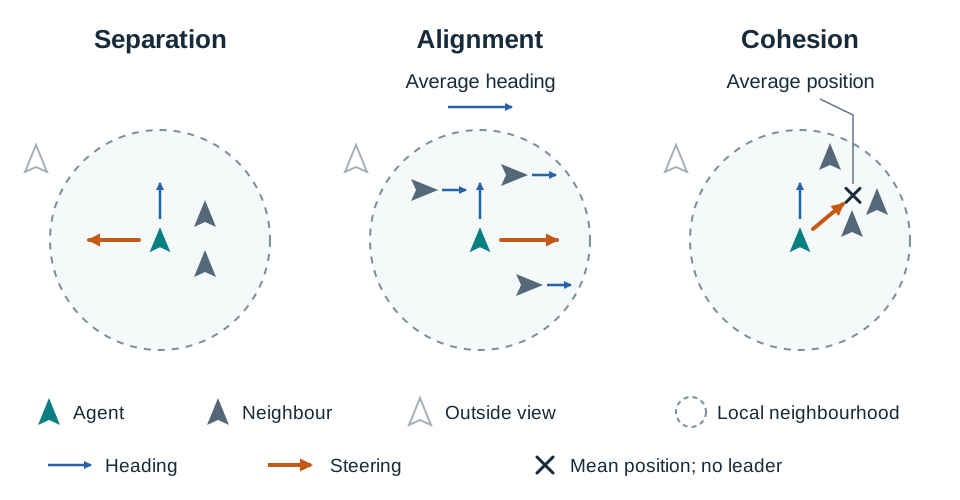
From these three simple rules, the fluid, swirling formation of a flock emerges naturally.
Another core example is an agent-based disease spread model. Each agent represents a person with an internal state (susceptible, infected, recovered), moves randomly, and applies one local rule: 'if I share a cell with an infected person, I become infected with probability '. No agent knows the global infection curve, yet the classic epidemic curve emerges from individual contacts, allowing scenarios such as 'vaccinate 50% of agents' to be tested.
Why Choose Agent-Based Modelling?
- No global equation is needed: Crowds, markets, and epidemics have no single mathematical formula, but individual rules are simple to define.
- Individuals can differ: Each agent can hold unique values for speed, health, or patience, capturing variety that top-down averages hide.
- Rules are easy to change and re-test: Modifying a local distance threshold or blocking a doorway requires changing only one rule.
- It reveals unexpected outcomes: Group behaviour is not hardcoded, so simulations often expose emergent bottlenecks or backward-travelling traffic jams.
- It is easy to visualise and explain: Showing moving agents on a screen is far more intuitive to non-technical stakeholders than presenting abstract equations.
- It scales: The same fundamental rules can simulate 20 agents or 20,000 agents.
Heuristics and Their Limitations (Higher Level)
According to the official specification, a heuristic is an approach to problem solving which aims to make an approximate solution to the problem. This can be used when time and resources are limited. The solution 'may not be feasible using classic or standard methods'. In plain terms: solving the problem exactly by the standard method would take too long or cost too much, so the heuristic aims to get as close to the best answer as it can.
We turn to heuristics when problems suffer from combinatorial explosion, where the number of possible solutions grows factorially or exponentially, making brute-force calculation impossible. In the Travelling Salesperson Problem (TSP) with 20 stops (a depot and 19 shops), an exhaustive brute-force search must evaluate:
Checking a billion routes per second would take roughly two years. A nearest-neighbour heuristic ('always visit the closest unvisited location next') returns a good route in milliseconds.
When to Reach for a Heuristic
Use a heuristic when all or most of these apply:
- The number of possible solutions is so vast that checking them all is impossible in reasonable time (route planning, timetabling, bin packing).
- A good answer now is worth more than a perfect answer later (a satnav calculating a detour while driving).
- The exact method exists but requires more computing power or memory than is available.
- The input data is already approximate (forecast traffic or weather), so an exact calculation gives false precision.
- A small error has a minor consequence (a delivery route 3% longer than optimal still delivers every package).
When a Heuristic Should Be Avoided
- Where an exact answer is legally or financially required: payroll calculations, tax, banking balances, and exam marking.
- In safety-critical systems where an approximation could cause injury: aircraft fuel margins, radiotherapy dosage.
- Where the exact method is already fast enough: sorting small lists or searching indexed databases.
- Where a sub-optimal answer cannot be detected or corrected afterwards.
Syllabus Limitations of Heuristics
The official specification defines four explicit trade-offs. Using a heuristic may involve the loss of:
- Precision: The result is rounded or grouped into bands.
- Accuracy: The output deviates from the true real-world figure.
- Optimal performance (optimality): The solution found is practical, but not guaranteed to be the best possible.
- Completeness: The algorithm might fail to find a solution even if one exists, or get trapped in local optima.
Applied Learning Task 3 and Assessment Context
In Applied Learning Task 3 (ALT 3), you collaborate to develop a computer system that simulates or models a problem that is difficult to solve analytically.
Your report on this task should be structured around the design process the specification sets out: Investigate → Plan → Design → Create → Evaluate → Document, with iteration running across the whole cycle. You are expected to loop back — evaluating a scenario usually sends you back to redesign a rule or fix a bug before you document the final version. Submitting the first version that runs, with no re-testing, is exactly what the coursework criteria describe as a low level of achievement.
The strand 3 applied learning tasks are team-based and are not marked by the SEC. Your artefact and individual report go into your digital portfolio, and both you and your teacher must verify that the task is completed. Separately, in term 1 of sixth year the SEC sets a coursework brief (30% of the marks, about 10 weeks to complete) which must be done individually, not in a group. The modelling skills you build in this task are examined in two places: in that coursework, and in the written and practical questions of the end-of-course examination.
Key terms
- Model
- A simplified representation of a real-world object, system, or process that captures essential features while omitting irrelevant details.
- Simulation
- The execution of a computational model over time to observe dynamic behaviours, track changing variables, and evaluate system responses.
- Abstraction
- The computational thinking practice of removing or hiding unnecessary details to focus exclusively on essential characteristics.
- Abstract Model
- A conceptual, visual, or mathematical representation that simplifies reality by explicitly retaining relevant variables and discarding irrelevant ones.
- Scenario
- A specific set of starting conditions, input variables, and parameters configured for a simulation run.
- Analytical Solution
- An exact mathematical solution calculated directly using standard formulas or closed-form equations without running a step-by-step simulation.
- Time Step
- The fixed slice of discrete simulated time processed during one complete pass of a simulation loop.
- Deterministic Simulation
- A simulation governed by fixed rules that always produces identical outputs when executed with identical starting inputs.
- Stochastic Simulation
- A simulation that incorporates pseudo-random variables, meaning individual runs with identical initial parameters produce varying results.
- Agent-Based Modelling
- A bottom-up simulation technique where autonomous entities (agents) interact according to simple local rules within an environment.
- Agent
- An individual autonomous entity in an agent-based model that maintains an internal state and acts using a limited local view.
- Emergent Behaviour
- Complex macro-level patterns that arise spontaneously from the local interactions of autonomous agents without central coordination.
- Heuristic
- An approximate problem-solving approach used when time and resources are limited, trading off precision, accuracy, optimal performance, or completeness.
- Verification
- The testing process of determining whether software code executes its intended rules correctly without bugs or logic errors.
- Validation
- The process of determining whether a model's outputs accurately reflect the behaviour of the real-world system being investigated.
Check yourself
Write two lines of Python that simulate one roll of a six-sided die and print the result.
python
from random import randint
print(randint(1, 6))
Write an if statement in Python that carries out an action with a probability of 0.25.
python
from random import random
if random() < 0.25:
    print("Event happened")   # replace with the action you need
What is the primary difference between a model and a simulation?
A model is an abstract representation containing the rules, data, and constraints of a system; a simulation is the active execution of that model over time.
State the simple retention hook that distinguishes verification from validation.
Verification asks 'did I build the thing right?' (checks code for bugs), while validation asks 'did I build the right thing?' (checks if results match reality).
What three local rules produce emergent flocking behaviour in Craig Reynolds' Boids model?
Separation (steer to avoid crowding neighbours), alignment (steer towards average heading of neighbours), and cohesion (steer towards average position of neighbours).
According to the official curriculum specification, what four qualities may be lost when using a heuristic?
A heuristic may involve the loss of precision, accuracy, optimal performance (optimality), or completeness.
In a queue simulation where queue = 2, arrivals = 3, and service capacity = 8, what is the new queue length?
Available = 2 + 3 = 5. Served = min(5, 8) = 5. New queue = 5 - 5 = 0 students.