

An algorithm is a finite, unambiguous sequence of steps designed to solve a problem or perform a task. In Leaving Certificate Computer Science, you need to understand how algorithms are built using sequence, selection, and iteration, represent them using flowcharts and pseudocode, trace them systematically using trace tables, write them in Python, and evaluate their efficiency using Big O notation. This topic covers the two required searching algorithms (linear search and binary search), the four sorting algorithms named on the course (simple sort, insertion sort, bubble sort, and quicksort), recursive functions, and the practical role and limitations of heuristics.
Algorithm Representation: Flowcharts, Pseudocode, and Trace Tables
An algorithm takes input data, processes it through logical steps, and produces an output. A good algorithm should be finite (it must stop after a finite number of steps), unambiguous (each instruction is clear and precise), and provide a general solution (it works correctly for any valid input, regardless of data values or input size).
All algorithms rely on three fundamental constructs:
- Sequence: executing instructions in order, one after another.
- Selection: making decisions based on conditions using
if,elif, andelse. - Iteration: repeating instructions using loops such as
forandwhile.
Flowcharts
A flowchart represents an algorithm visually using standard geometric shapes:
- Oval (terminator): marks the START or STOP of the program.
- Parallelogram: represents INPUT or OUTPUT operations.
- Rectangle (process): represents a calculation or data assignment (such as
total = total + n). - Diamond (decision): asks a condition with two branch exits, labelled TRUE/FALSE or YES/NO.
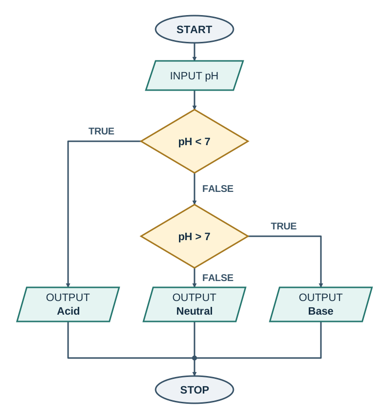
When a problem requires multiple conditions (for example, categorising a chemical solution as acid, base, or neutral), decisions connect sequentially. The FALSE branch of the first test (pH < 7) leads directly into the second test (pH > 7). The final output on the second FALSE branch represents the default case (Neutral).
Pseudocode and Trace Tables
Pseudocode expresses algorithmic logic in structured plain English without requiring specific programming language syntax.
SET total TO 0
SET count TO 0
WHILE count < 3
    INPUT n
    total = total + n
    count = count + 1
END WHILE
OUTPUT total / count
A trace table allows you to track and record the value of every variable after each step, verifying program behaviour before running the code.
| Step / Input | n | total | count | count < 3? | Output |
|---|---|---|---|---|---|
| Initialisation | 0 | 0 | 0 | True | |
| Input 5 | 5 | 5 | 1 | True | |
| Input 10 | 10 | 15 | 2 | True | |
| Input 6 | 6 | 21 | 3 | False | |
| Termination | 6 | 21 | 3 | 7.0 |
The loop ends when count reaches 3. The output is 21 / 3 = 7.0 (in Python, standard division / yields a floating-point number).
Algorithmic Complexity and Big O Notation
Rather than timing code in seconds—which changes depending on the computer processor used—we measure algorithmic efficiency using Big O notation. Big O describes how an algorithm's running time or memory usage scales as the input size increases.
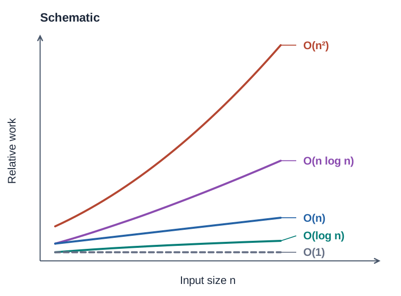
To see why this matters, consider input growth: if a list grows from 10 to 100 items ( larger), an algorithm performs 10 times more operations, while an algorithm performs times more operations.
| Complexity | Name | How Operations Grow | Example |
|---|---|---|---|
| Constant Time | Unaffected by input size | Reading a list element at a known index (L[0]) | |
| Logarithmic Time | Halves the remaining data space at each step | Binary search on a sorted list | |
| Linear Time | Grows directly in proportion to | Linear search across a list | |
| Log-Linear Time | Divides data efficiently while recombining | Quicksort in best and average cases | |
| Quadratic Time | Grows with the square of ; doubling quadruples work | Nested loops in bubble sort, simple sort, insertion sort |
Complexity is evaluated across three conditions:
- Best case: the minimum number of steps needed under ideal input conditions.
- Average case: the typical number of operations required for randomly ordered data.
- Worst case: the maximum number of operations required for the least favourable data arrangement.
Searching Algorithms: Linear and Binary Search
Searching algorithms find the position of a target item in a list.
Linear Search
Linear search examines each item sequentially from index 0 until the target is located or the list ends. It works on unsorted and sorted lists alike.
# Using a while loop with a found flag
names = ["John", "Mary", "Zoe", "Alex", "Séamas"]
target = "Zoe"
found = False
index = 0

while not found and index < len(names):
    if names[index] == target:
        found = True
    else:
index += 1- Best case: 1 comparison (target is at index 0), so .
- Average case: checks roughly half the list ( steps), so .
- Worst case: comparisons (target is the last item or absent), so .
Binary Search
Binary search works by repeated halving. It compares the target with the middle element. If the target matches, the search ends; if smaller, the search continues in the left half; if larger, it continues in the right half. The essential prerequisite is that the list must be sorted.
def binary_search(numbers, target):
    low = 0
    high = len(numbers) - 1
    while low <= high:
        mid = (low + high) // 2
        if numbers[mid] == target:
            return mid
        elif numbers[mid] < target:
            low = mid + 1
        else:
            high = mid - 1
    return -1  # Target not in list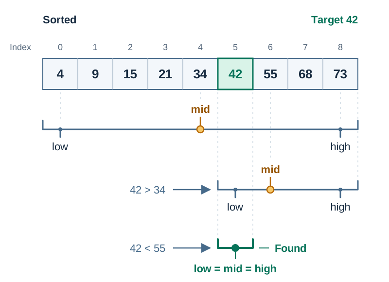
- Best case: 1 comparison (target is at the initial midpoint), so .
- Average and worst case: halving means a list of size takes roughly comparisons, so .
Each doubling of the list size adds just one comparison. A list of 1,000 items takes at most 10 comparisons (), while 1,000,000 items takes only about 20 comparisons.
If you only need to run a single search on an unsorted list, linear search () is faster overall than sorting first () just to run a binary search. If you need to search the same data repeatedly, sorting it once and using binary search saves time.
Simple Sort and Insertion Sort
Sorting organizes items into ascending or descending order. The data elements must be comparable.
Simple Sort (often taught as Selection Sort)
The syllabus lists 'Simple sort'. In classroom practice, simple sort is usually taught as repeatedly finding the smallest remaining item in the unsorted section and placing it into its correct position at the front, which is identical to selection sort.
def simple_sort(numbers):
    n = len(numbers)
    for i in range(n):
        min_index = i
        for j in range(i + 1, n):
            if numbers[j] < numbers[min_index]:
                min_index = j
        numbers[i], numbers[min_index] = numbers[min_index], numbers[i]
    return numbers
Trace on [29, 10, 14, 37, 13]:
- Pass 1: find minimum (10), swap with index 0
[10, 29, 14, 37, 13] - Pass 2: find minimum from index 1 (13), swap with index 1
[10, 13, 14, 37, 29] - Pass 3: find minimum from index 2 (14), already at index 2
[10, 13, 14, 37, 29] - Pass 4: find minimum from index 3 (29), swap with index 3
[10, 13, 14, 29, 37]
Simple sort scans every unsorted item in every pass, so best, average, and worst cases are all .
Insertion Sort
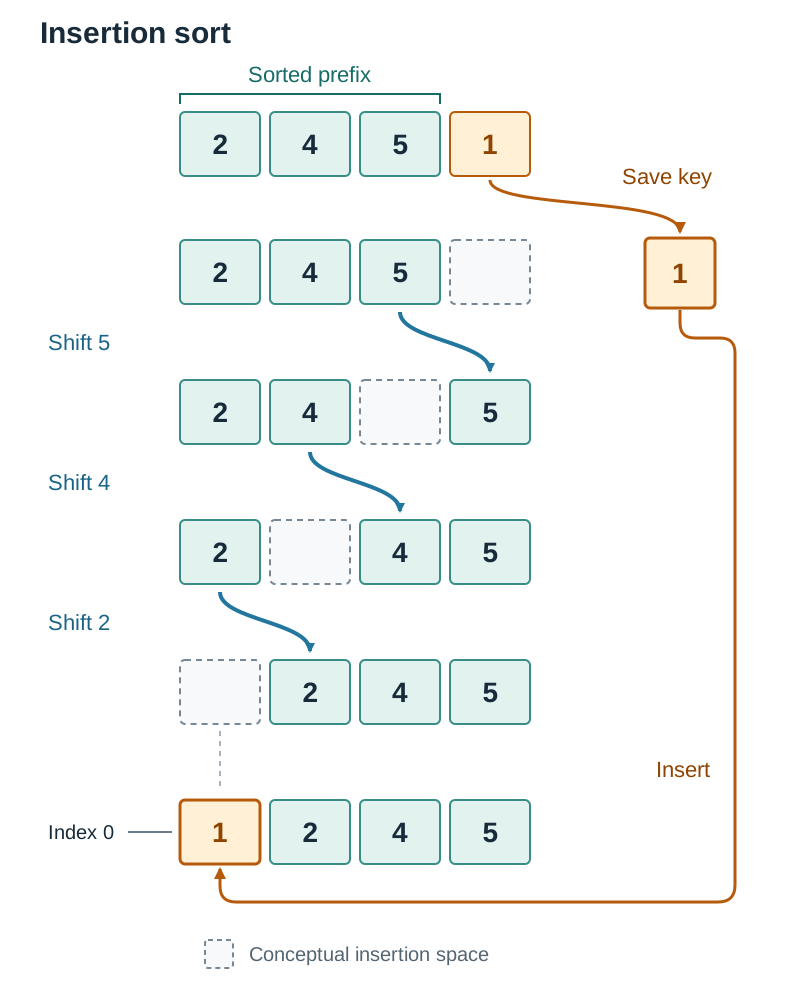
Insertion sort mimics sorting a hand of playing cards. It steps through the list, picks the next item (the key), and shifts larger items in the sorted portion one slot to the right until the key reaches its place.
def insertion_sort(numbers):
    for i in range(1, len(numbers)):
        key = numbers[i]
        j = i - 1
        while j >= 0 and numbers[j] > key:
            numbers[j + 1] = numbers[j]  # Shift right
            j -= 1
        numbers[j + 1] = key
    return numbers
Trace on [5, 2, 4, 1]:
- , key = 2: , shift 5, insert 2
[2, 5, 4, 1] - , key = 4: , shift 5, stop before 2, insert 4
[2, 4, 5, 1] - , key = 1: shift 5, 4, and 2, insert 1 at index 0
[1, 2, 4, 5]
- Best case: when the list is already sorted. Each item is compared once with its neighbour on the left, requiring 0 shifts.
- Average and worst case: . A reversed list requires comparing and shifting past every item in the sorted section.
Bubble Sort
Bubble sort steps through a list, compares adjacent items, and swaps them if they are out of order. With each complete pass, the largest remaining item moves to the end of the unsorted segment.
def bubble_sort(numbers):
    n = len(numbers)
    for i in range(n):
        swapped = False
        for j in range(0, n - i - 1):
            if numbers[j] > numbers[j + 1]:
                numbers[j], numbers[j + 1] = numbers[j + 1], numbers[j]
                swapped = True
        if not swapped:
            break  # Early exit if no swaps occurred
    return numbers
Understanding Bubble Sort Complexity
The best-case complexity depends on whether the code includes an early-exit flag:
- Basic Bubble Sort (no flag): runs every pass regardless of order. It performs roughly comparisons on every list, meaning its best and worst cases are both .
- Optimised Bubble Sort (with
swappedflag): stops after one pass if no swaps are made. On an already sorted list, it makes comparisons and terminates, giving a best-case complexity of . - In the worst case (a reverse-sorted list), both versions make the maximum number of comparisons and swaps: .
Recursion and Quicksort
A recursive function is a function that calls itself to solve smaller instances of the same problem. Every recursive algorithm requires two components:
- A base case, which stops recursion and returns a result directly without another call.
- A recursive case, which calls the function again with inputs closer to the base case.
def factorial(n):
    if n <= 1:          # Base case
        return 1
    return n * factorial(n - 1)  # Recursive case
Tracing factorial(4):
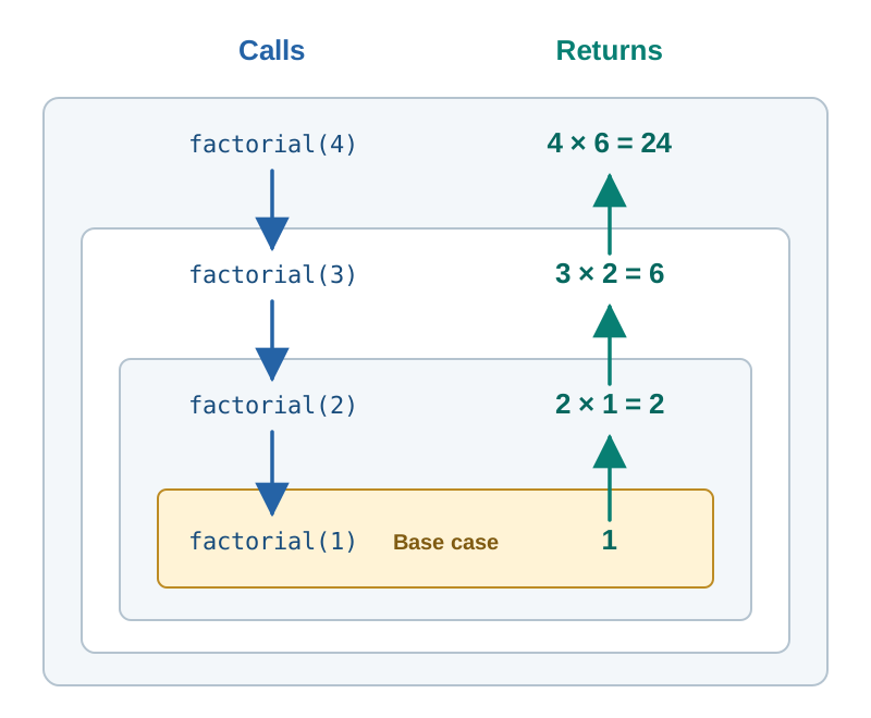
factorial(4)waits forfactorial(3)waits forfactorial(2)waits forfactorial(1)hits the base case and returns 1.
The pending calls resolve backwards: , then , then . If the base case is missing or never reached, the program will trigger a RecursionError by exceeding Python's call limit.
Quicksort
Quicksort is a divide-and-conquer algorithm. It selects an item as a pivot, creates sublists of items smaller than, equal to, and greater than that pivot, and sorts the smaller and larger sublists recursively.
def quicksort(numbers):
    if len(numbers) <= 1:      # Base case
        return numbers

    pivot = numbers[len(numbers) // 2]
    left = [x for x in numbers if x < pivot]
    middle = [x for x in numbers if x == pivot]
    right = [x for x in numbers if x > pivot]

    return quicksort(left) + middle + quicksort(right)
Pivot Selection and Partition Balance
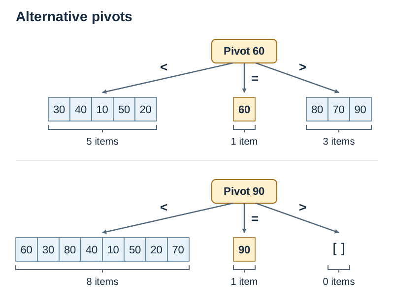
- Best and average case: . Occurs when the pivot divides the list into roughly equal halves, producing a balanced recursion tree.
- Worst case: . Occurs when the pivot is repeatedly the extreme smallest or largest element. This produces an unbalanced partition where one sublist contains items and the other contains 0, eliminating the advantage of divide-and-conquer.
For example, in the list [60, 30, 80, 40, 10, 50, 20, 70, 90], picking 90 as the pivot places all 8 other items into the left sublist and leaves the right sublist empty, creating a worst-case partition.
Comparing Algorithms and Using Heuristics
Choosing the right algorithm depends on data size, whether the data is already ordered, and memory constraints.
| Algorithm | Advantages | Limitations |
|---|---|---|
| Linear Search | Simple to code; works on unsorted data | Slow on large datasets: worst case |
| Binary Search | Fast on large datasets: | Data must be sorted first; harder to write |
| Simple Sort | Easy to trace; makes at most swaps | Always comparisons, even if sorted |
| Insertion Sort | Fast on nearly sorted lists: best case ; sorts in place | Average and worst case are |
| Bubble Sort | Simple logic; early-exit flag detects sorted lists | Slow in practice: makes many swaps; worst case |
| Quicksort | Very fast on large datasets: average | Degrades to with poor pivots; recursive calls use call-stack memory |
Heuristics
Some problems have so many combinations that checking every possibility would take years, even on supercomputers. For example, in the Travelling Salesperson Problem (finding the shortest route visiting cities), 20 cities produce more than different possible routes, far too many to check one by one.
When calculating an exact answer is impractical, computer scientists use a heuristic: a practical problem-solving method designed to find a good-enough solution quickly.
- Nearest Neighbour Heuristic:
- Start at any city.
- Always visit the closest unvisited city next.
- When all cities have been visited, return to the start.
This delivers a usable route in seconds. However, because each local decision is made without seeing the full map, an early choice might force a long leg at the end.
- When to use heuristics: when computing resources or time are limited, and an approximate answer is acceptable (such as sat-nav routing, video game AI, or delivery scheduling).
- When to avoid heuristics: when an exact, guaranteed answer is mandatory (such as banking transactions, cryptography, or medical drug dosages).
- Trade-offs: using a heuristic can involve a loss of precision, accuracy, optimal performance, or completeness.
Key terms
- Algorithm
- A finite, unambiguous sequence of steps designed to accomplish a specific task or solve a computational problem.
- General Solution
- A solution that applies to different situations and inputs, consistently producing the correct output regardless of the size or specific values of the input data.
- Big O Notation
- A mathematical notation used to classify algorithms according to how their execution time or memory requirements scale as input size increases.
- Linear Search
- A search algorithm that examines each element in a collection sequentially from start to finish until a match is found or the list ends.
- Binary Search
- A search algorithm that repeatedly halves the search space of a sorted list by comparing the target value to the midpoint element.
- Simple Sort
- A comparison sort named on the syllabus, commonly implemented as selection sort, which repeatedly selects the minimum unsorted item and places it into the next position.
- Insertion Sort
- A sorting algorithm that builds an ordered list by taking unsorted elements one at a time and inserting them into their correct position by shifting larger elements.
- Bubble Sort
- A sorting algorithm that steps through a list, compares adjacent elements, and swaps them if they are in the wrong order.
- Quicksort
- A divide-and-conquer sorting algorithm that partitions a list into sublists around a selected pivot element and sorts each sublist recursively.
- Recursion
- A programming technique where a function calls itself to solve a smaller instance of the same problem until it reaches a base case.
- Base Case
- The condition in a recursive function that terminates recursion by returning a direct value without making further recursive calls.
- Heuristic
- An approach to problem solving that aims to produce an approximate, practical solution when finding an optimal solution is unfeasible due to time or resource constraints.
Check yourself
What does it mean to say that an algorithm provides a 'general solution'?
It means the algorithm can be applied to different inputs and will always produce the correct output, regardless of the specific values or the size of the input.
A student searches a mystery list by first checking if the value is >= 4, halving the possibilities, while another checks 1, 2, 3 in order. Name both search methods and identify which is more efficient.
Halving the possibilities is binary search; checking sequentially is linear search. Binary search is more efficient because it has a complexity of O(log n), halving remaining items each step, whereas linear search checks items one by one with a complexity of O(n).
Show the list [8, 5, 9, 7, 6] after each of the first three passes of bubble sort.
Pass 1: [5, 8, 7, 6, 9]. Pass 2: [5, 7, 6, 8, 9]. Pass 3: [5, 6, 7, 8, 9].
What are the two mandatory components that every recursive function must contain?
A base case (which ends recursion and returns a result directly) and a recursive case (which calls the function again with an input closer to the base case).
Name the four specific trade-offs or losses that may occur when using a heuristic according to the curriculum specification.
Loss of precision, accuracy, optimal performance, or completeness.