

In Climate Action and Sustainable Development, secondary data refers to pre-existing information collected, validated, and published by external scientific bodies, government agencies, and historical records. Because monitoring global climate systems requires vast networks of calibrated weather stations, satellite constellations, ocean buoys, and paleoclimate proxy records operating over centuries, climate science relies fundamentally on secondary data. Strand 1 (Learning Outcome 1.7) requires you to demonstrate the evidence for human-induced (anthropogenic) global warming across five distinct lines of secondary data: atmospheric greenhouse gas levels, surface and ocean temperature changes, precipitation patterns, sea level rise, and historical or oral testimony. Mastering this topic means moving beyond basic graph reading. You need to extract exact figures with units, calculate percentage changes and rates, evaluate source credibility and data limitations, join independent lines of evidence into a causal chain, and apply the Data-Explain-Implication answering structure across the written examination and the coursework Action Project.
Assessment Structure and Secondary Data in Climate Science
Assessment Structure at a Glance
Assessment for certification in Leaving Certificate Climate Action and Sustainable Development is split into two components:
- Written Examination (60%, 300 marks): Assessed at Higher Level across three sections: Section A (60 marks), Section B (160 marks), and Section C (80 marks). Stimulus-based data questions can appear anywhere across these sections.
- Action Project (40%, 200 marks): An individual digital journal based on an SEC common brief (the 2027 brief focus is Reducing Ireland's Greenhouse Gas Emissions). The journal has an upper limit of 1,800 words and up to 10 images.
Primary versus Secondary Data
- Primary data is information you collect yourself first-hand in the field. Carrying out a kick-sample to record macroinvertebrates in a local stream, measuring soil compaction with a penetrometer, or surveying commuting habits in your school generates primary data.
- Secondary data is information collected, processed, and published by someone else that you retrieve and repurpose for an investigation.
Secondary datasets appear in two formats: quantitative data (numerical measurements such as atmospheric gas concentrations in parts per million or national sectoral emissions in kilotonnes of carbon dioxide equivalent, ) and qualitative data (descriptive, non-numerical accounts such as archival harvest records or oral testimony from coastal communities).
Advantages of Secondary Data
- It covers geographical scales and time spans no individual or school could measure, including 800,000-year ice-core records, 65 years of continuous daily atmospheric sampling, and planetary satellite coverage.
- It is quality-assured: statutory agencies and research institutes calibrate sensors, publish peer-reviewed methodology, and correct instrumental drifts.
- It is efficient to retrieve, allowing researchers and students to direct time towards analysis, planning, and taking informed local action.
- It enables standardized comparison against internationally agreed historical baselines.
Limitations of Secondary Data
- It was gathered for another agency's purpose, so it may not answer your exact question (for example, national emissions data rarely provides a county- or school-level breakdown).
- It is frequently aggregated into regional averages or national totals, masking local variations.
- It can be subject to reporting lags or published as provisional data that is revised a year later (such as EPA annual emissions inventories).
- Because you did not oversee data collection, you must check the measurement method, baseline period, and margin of error before accepting findings.
- Some sources present selective or biased data to support commercial or political agendas.
Analytical Toolkit: Reading Stimuli, Baselines, and Calculations
Reading the Stimulus Step-by-Step
Before writing an exam answer or citing coursework figures, examine the data stimulus methodically:
- Check the title, agency, and publication date to establish what is measured and whether the source is authoritative.
- Read both axes carefully, checking the variable, unit, and any multiplier (such as , , or ).
- Check the time span and baseline reference period. A five-year window shows weather fluctuations; a climate signal requires multi-decadal observation.
- Identify whether the visual is a line graph, bar chart, or a stacked area chart.
Describing Trends Correctly
- State the overall trend in one sentence with initial and final figures and units. A trend is a sustained long-term direction; do not confuse it with a short-term fluctuation (an isolated annual dip or spike).
- Quantify the change by stating the absolute change, percentage change, or annual rate.
- Identify notable turning points, peaks, or dips, noting the specific year (for example, the sharp drop in transport emissions in 2020 due to Covid-19 travel restrictions).
Baselines and Climate Anomalies
Raw absolute temperatures vary greatly with altitude and local topography. Climatologists express measurements as anomalies to eliminate local geographic offsets and calculate true planetary shifts. A climate anomaly is the mathematical difference between an observed value and the long-term average calculated over an agreed baseline period:
Two baseline types are standard in climate science:
- Pre-industrial baseline (1850–1900): A 51-year reference period used to evaluate total global warming since industrialisation began (for example, stating that the planet has warmed by roughly 1.1 °C to 1.3 °C).
- 30-year climate normal: Standard multi-decadal reference windows (such as 1961–1990 or 1991–2020) used by Met Éireann and the WMO to evaluate recent regional weather against recent historical averages.
Essential Mathematical Calculations
- Absolute Change ():
- Percentage Change:
Always divide by the starting value, not the final value.
- Average Annual Rate of Change:
- Sector Share of National Total:
Critical Technical Distinctions
- Stock versus Flow: Atmospheric concentration is a cumulative stock (measured in ppm or ppb), representing total gas residing in the atmosphere. Emissions are an annual flow (mass released per year, such as ). Reducing annual emissions reduces the inflow, but atmospheric concentrations will continue to rise as long as annual emissions exceed natural absorption sinks.
- Percent versus Percentage Points: If a sector's emissions share shifts from 20% to 25%, that represents a rise of 5 percentage points, but a relative increase of 25% ().
- Reading Stacked Area Charts: In a stacked graph (such as the EPA emissions by sector chart in the 2027 Action Project brief), calculate a sector's emission value by measuring the vertical distance between its upper and lower boundary lines; do not read the top line against the vertical axis.
The Five Pillars of Anthropogenic Evidence
Strand 1 Learning Outcome 1.7 requires you to demonstrate the evidence for human-induced global warming across five specific categories of secondary data.
1. Atmospheric Greenhouse Gas Concentrations
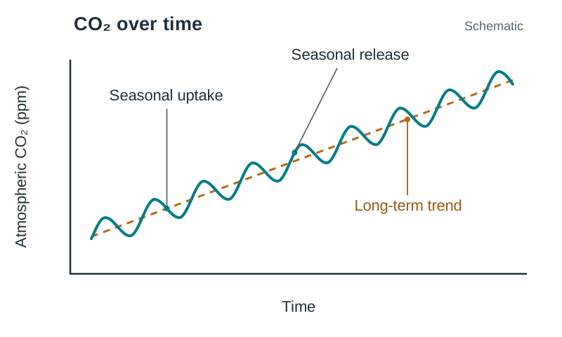
Direct continuous measurements from the Mauna Loa Observatory in Hawaii (the Keeling Curve) show atmospheric carbon dioxide () increasing from approximately in 1958 to over today. The record rises steadily year on year while exhibiting an annual zig-zag pattern. This annual oscillation reflects the seasonal cycle of Northern Hemisphere land vegetation, which absorbs through photosynthesis during spring and summer and releases it as deciduous matter decays during autumn and winter.
To contextualise modern gas levels before instrumental records began, scientists examine proxy data from air bubbles trapped in polar ice cores (such as EPICA Dome C in Antarctica). These show that for 800,000 years, atmospheric fluctuated naturally between during ice ages and during warm interglacial intervals. Today's concentration exceeds , over 40% higher than the pre-industrial peak.
Atmospheric concentrations of other gases show similar climbs:
- Methane (): Risen from a pre-industrial baseline of roughly to over today, driven by enteric fermentation in ruminant livestock, fossil fuel extraction, and landfills. Methane is measured in parts per billion (ppb).
- Nitrous Oxide (): Risen from roughly to around , primarily from synthetic nitrogen fertilisers and animal manure management.
Scientists can also determine where the extra atmospheric carbon originates: carbon from ancient fossil fuels has a distinct chemical signature (a lower ratio of Carbon-13 to Carbon-12) compared to carbon cycled through living plants, and the atmospheric signature matches fossil fuel combustion.
2. Surface and Ocean Temperature Change
Global temperature compilations (including NASA GISTEMP and HadCRUT) show global mean surface temperatures have risen by roughly to above the pre-industrial baseline (1850–1900). Each decade since 1980 has been warmer than the previous one. In Ireland, Met Éireann records from long-running stations like Valentia Observatory, Co. Kerry, and the Phoenix Park, Dublin, show that Ireland's average annual temperature has increased by roughly over the past 120 years. Armagh Observatory in Northern Ireland holds meteorological observations dating back to 1795, providing long-term island-of-Ireland corroboration. Oceanographic data confirms that the upper oceans absorb over 90% of the planetary energy imbalance.
3. Global Precipitation Regimes
Under the Clausius-Clapeyron relation, every of atmospheric warming allows air to hold roughly 7% more water vapour. This intensifies hydrological cycles, resulting in heavier precipitation events. Met Éireann secondary data reveals that average annual rainfall in Ireland for 1989–2018 was roughly 6–7% higher than the 1961–1990 average, characterised by heavier winter rainfall and greater frequency of summer soil moisture deficits.
4. Rising Sea Levels
Tide-gauge records combined with satellite altimetry data operating since 1993 demonstrate that global mean sea level rose by roughly between 1901 and 2018. The rate of rise accelerated from roughly across the twentieth century to over in recent decades. Physics secondary data attributes this rise to two main drivers: thermal expansion (ocean water physically expands as it warms) and land ice melt (water entering oceans from melting glaciers and the Greenland and Antarctic ice sheets). Note that melting floating sea ice does not directly alter sea level because it already displaces its own volume of water.
5. Historical and Indigenous Testimony
Qualitative documentary archives and oral traditions cross-reference physical instrumental records. The Kyoto cherry blossom records in Japan, which track the annual peak bloom date back to 801 AD, recorded their earliest peak flowering in over 1,200 years in 2021. Century-long French vineyard records show harvest dates occurring progressively earlier in the calendar year, reflecting higher spring temperatures. Indigenous Arctic oral histories document thinning seasonal sea ice and changes in wildlife migration that corroborate satellite observations.
Summary Table: Evidence Types, Datasets, and Specific Limitations
| Indicator | Named Dataset / Source | Key Quantified Figure | Inherent Limitation to Name in Exam |
|---|---|---|---|
| Atmospheric | Keeling Curve (Mauna Loa) & Antarctic Ice Cores | (1958) to today; pre-industrial range | Direct instrumental readings date only from 1958; pre-1958 values rely on ice cores where air bubbles seal over decades, giving lower time resolution. |
| Surface Temperature | NASA GISTEMP / HadCRUT / Met Éireann | to globally; in Ireland over 120 years | Pre-1950 weather stations were sparse in the Southern Hemisphere and oceans; urban growth around stations requires mathematical corrections (homogenisation) that introduce margins of error. |
| Precipitation | Met Éireann national station networks | Irish rainfall up roughly 6–7% (1989–2018 vs 1961–1990 baseline) | High local and annual variability means short records can hide long-term trends; rain gauges under-catch precipitation in high-wind conditions. |
| Sea Level | Coastal Tide Gauges & Satellite Altimetry | Total rise since 1901; current rate | Tide gauges measure sea level relative to local land that may be naturally subsiding or rising; satellite radar altimetry records only begin in 1993. |
| Historical Testimony | Kyoto Bloom Logs / French Grape Harvests / Indigenous Oral Histories | Kyoto peak bloom in 2021 was the earliest recorded in years | Qualitative and subjective; records survive unevenly; harvest and flowering dates can be affected by local land-management changes rather than temperature alone. |
The Causal Chain and Ruling Out Natural Forcings
At Higher Level, demonstrating human causation requires showing physical mechanism rather than relying on correlation (two graphs moving upward together). To prove causation, you must link independent datasets into a structured chain:
- Emissions and Concentrations: Secondary records show atmospheric concentrations of , , and rising sharply since 1750, matching historical emission totals from fossil fuel combustion, agriculture, and industrial development.
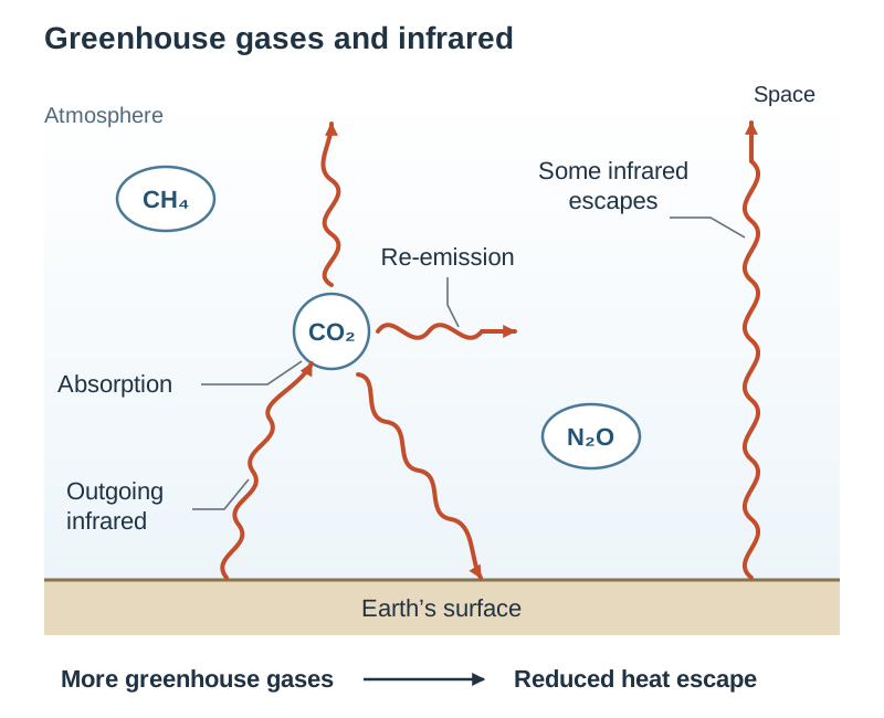
- Physical Mechanism: The enhanced greenhouse effect is an established principle of atmospheric physics. Greenhouse gas molecules absorb outgoing long-wave infrared radiation emitted by Earth's surface and re-radiate thermal energy in all directions, reducing the rate at which heat escapes into space.
- Observed Planetary Warming: Long-term surface and ocean temperature measurements confirm warming that tracks greenhouse gas accumulation over multi-decadal scales.
- Thermodynamic Consequences: Physical impacts match scientific predictions: seawater expands as it warms, land ice melts, sea levels rise, and warmer air holds more moisture, leading to altered precipitation regimes.
- Ruling Out Natural Drivers: Climatologists use secondary monitoring data to test and eliminate alternative natural explanations:
- Solar Irradiance: Satellite monitoring shows total solar irradiance has remained flat or declined slightly since about 1980, even while global temperatures have climbed. Furthermore, solar warming would heat the entire atmosphere equally; secondary satellite and weather balloon data show the lower atmosphere (troposphere) warming while the upper atmosphere (stratosphere) cools. This cooling stratosphere is the distinct signature of greenhouse gases trapping heat near the surface.
- Volcanic Activity: Explosive volcanic eruptions (such as Mt Pinatubo in 1991) inject sulphate aerosols into the stratosphere. These reflect incoming solar radiation, causing temporary global cooling for 1 to 3 years. They do not cause sustained multi-decadal warming.
Evaluating Sources and Using Data in the Action Project
Evaluating Data and Spotting Manipulation
The specification glossary defines Evaluate (data) as examining data to make judgements and appraisals, describing how evidence supports or refutes a conclusion, and identifying limitations in findings. When assessing secondary sources in the written exam or in Section A of your coursework, check the material against key evaluation criteria:
- Who compiled the data?: Was it compiled by a recognised statutory agency (EPA, Met Éireann, CSO), a peer-reviewed research body, or an unverified campaign or commercial website?
- Transparency: Does the publisher clearly explain instrumentation, sampling frequency, margins of error, and the baseline reference period used?
- Vested Interests: Does the publisher have a financial or political motive to present a selective narrative?
- Cherry-picking: Selecting a short, unrepresentative timeframe or an anomalous baseline year to hide an overall trend (for example, starting a temperature chart in an exceptional heatwave year to make subsequent years appear to cool).
- Axis Truncation: Cutting off a vertical axis to visually exaggerate minor variations. For example, plotting Irish emissions on an axis starting at makes a 2% change appear as a dramatic collapse. Always inspect whether the vertical axis starts at zero.
Where to Source Irish Secondary Data for the 2027 Action Project
- Environmental Protection Agency (EPA): Publishes Ireland's official national greenhouse gas emissions inventories by sector, provisional annual figures, and 2030 projections.
- Sustainable Energy Authority of Ireland (SEAI): Provides energy balance statistics, tracking fossil fuel consumption and renewable energy penetration across electricity, transport, and heating.
- Met Éireann: Offers long-term temperature, rainfall, and sunshine records along with annual climate statements.
- Central Statistics Office (CSO): Compiles census data, vehicle registrations, agricultural livestock counts, and household heating types to explain why sectoral emissions change.
- Climate Change Advisory Council (CCAC): Issues annual reviews evaluating State progress against statutory carbon budgets.
- Local Authority Climate Action Plans: Detail greenhouse gas profiles and mitigation measures at county and city level.
Presenting Secondary Data in the Action Project Journal
- The Action Project Journal carries 200 marks (40% of certification). The total word limit is 1,800 words; exceeding this limit incurs penalties. Section A (Research to inform action) has a suggested allocation of 350 words (30 marks).
- In-text citations and the bibliography in Section D are not included in the 1,800-word count.
- You can include a maximum of 10 images (including charts, graphs, and tables). Images cannot be used to embed supplementary text. Video files are not permitted.
- Captured graphs must be clearly cited.
- No formal referencing style (such as Harvard or APA) is mandatory under NCCA guidelines, but your references must contain enough accurate detail to allow the reader to authenticate the source.
- Any use of artificial intelligence tools must be acknowledged, stating the tool name, date accessed, and the prompt or shareable link used.
Worked Citation Pair Example: (Example only; take your actual figure from the current EPA inventory)
- In-text citation in Section A:
...national emissions decreased by 4% in 2023, yet agriculture remained the largest emitting sector at 38% of the total (EPA, 2024). - Matching entry in Section D References:
Environmental Protection Agency (EPA) (2024), Ireland's Provisional Greenhouse Gas Emissions 1990-2023, epa.ie, accessed 14 October 2026.
Key terms
- Secondary Data
- Information collected, validated, and published by external organisations rather than gathered first-hand by the student or researcher.
- Quantitative Data
- Information expressed numerically as measurable quantities, such as atmospheric gas concentrations or emissions figures.
- Qualitative Data
- Descriptive, non-numerical information, such as oral histories, historical documentary chronicles, and observational testimonies.
- Baseline Period
- An agreed multi-decadal reference period (such as the 1850–1900 pre-industrial baseline or a 30-year climate normal) against which climate measurements and anomalies are calculated.
- Climate Anomaly
- The mathematical difference between an observed climate measurement and the long-term baseline average for that specific location and date.
- Keeling Curve
- The continuous daily record of atmospheric carbon dioxide concentration initiated at Mauna Loa Observatory in 1958.
- Proxy Data
- Preserved natural archives (such as ice cores, tree rings, and ocean sediment layers) used to reconstruct climatic conditions prior to modern instrumental monitoring.
- Enhanced Greenhouse Effect
- The additional warming of Earth's lower atmosphere caused by human emissions absorbing and re-radiating outgoing terrestrial infrared radiation.
- Thermal Expansion
- The increase in seawater volume that occurs as the oceans absorb planetary heat, serving as a primary physical driver of global sea level rise.
- Land Ice Melt
- The addition of water to oceans from grounded glaciers and continental ice sheets (Greenland and Antarctica), which raises global sea level.
- Clausius-Clapeyron Relation
- The physical relationship dictating that atmospheric moisture capacity increases by approximately 7% for every 1 °C of warming.
- Cherry-Picking
- The misleading practice of selecting narrow timeframes, isolated geographic areas, or anomalous baseline years to present a false impression that contradicts the broader trend.
- Axis Truncation
- The visual manipulation of a graph by not starting the vertical axis at zero, which artificially exaggerates or minimises visible changes.
- kt CO2 equivalent
- Kilotonnes of carbon dioxide equivalent; a metric standardising the global warming impact of various greenhouse gases relative to carbon dioxide.
- Stock
- The total cumulative quantity of a greenhouse gas residing in the atmosphere at any given time, measured in parts per million (ppm) or parts per billion (ppb).
- Flow
- The rate at which greenhouse gases are added to or removed from the atmosphere each year, measured in mass per unit time (such as kt CO2 eq/yr).
- Trend
- The sustained general direction of a variable observed over a multi-decadal timeframe.
- Fluctuation
- A short-term, temporary variation or anomaly that deviates from the long-term climatic trend.
Check yourself
What is the difference between direct instrumental climate data and paleoclimate proxy data?
Direct instrumental data consists of real-time measurements recorded by calibrated human sensors (such as thermometers and satellites), whereas proxy data consists of preserved biological or geological records (such as ice cores and tree rings) that indirectly reconstruct past climate.
What was the pre-industrial range of atmospheric carbon dioxide over the past 800,000 years, and what is the modern level?
Antarctic ice cores show that pre-industrial CO2 fluctuated between roughly 180 ppm during glacial periods and 280–300 ppm during warm interglacials. Today, direct measurements exceed 420 ppm.
A weather station records a mean annual temperature of 11.2 °C against a 1961–1990 baseline average of 9.7 °C. Calculate the temperature anomaly.
Anomaly = 11.2 °C - 9.7 °C = +1.5 °C.
Why does the Keeling Curve exhibit a regular intra-annual oscillation while climbing over the long term?
The annual oscillation reflects seasonal growth and decay of land vegetation in the Northern Hemisphere (absorbing CO2 in spring/summer and releasing it in autumn/winter), while the long-term upward climb is driven by fossil fuel combustion and land clearance.
How do satellite records of solar irradiance disprove the claim that recent warming is caused by the Sun?
Satellite records show total solar irradiance has remained flat or slightly declined since 1980 while global surface temperatures climbed. Furthermore, satellite observations show the troposphere warming while the stratosphere cools, which is the specific fingerprint of greenhouse gas trapping.
What are the two physical processes causing modern global sea level rise?
Thermal expansion of ocean water as it absorbs heat, and meltwater added from grounded glaciers and continental ice sheets in Greenland and Antarctica.
In a stacked sectoral emissions graph, how do you determine the emissions of a middle sector?
Calculate the vertical difference between that sector's upper boundary line and its lower boundary line; do not read the top boundary off the vertical axis.
Transport emissions were 10,900 kt CO2 eq in 2005 and 11,900 kt CO2 eq in 2023, when national emissions totalled 55,000 kt CO2 eq. Calculate the percentage change in transport emissions and transport's share of the 2023 national total.
Percentage change = ((11,900 - 10,900) / 10,900) 100 = +9.17%. Sector share = (11,900 / 55,000) 100 = 21.64%.